Overview (What I've Learned)
The goal of this project was to explore image warping beyond the simple translations we've done so far for 2 cool applications: 1.) Image Rectification and 2.) Image Mosaicing. In this project I captured images on my phone, calculated homography matrices mapping 2 images to each other, applied both forward inverse warping for transformation and finally alpha blended to stitch images together.
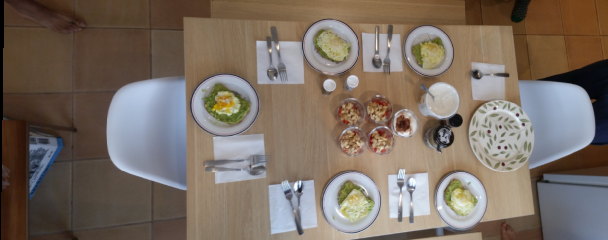
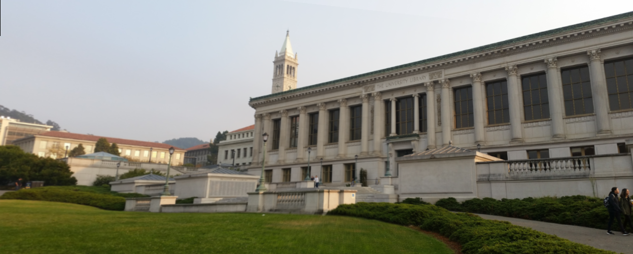
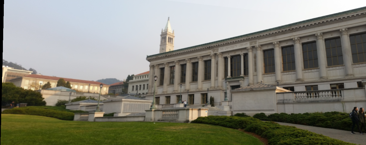
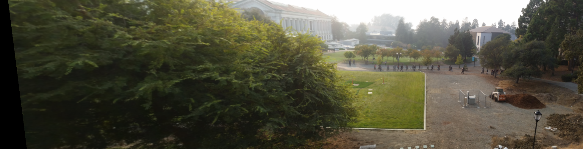
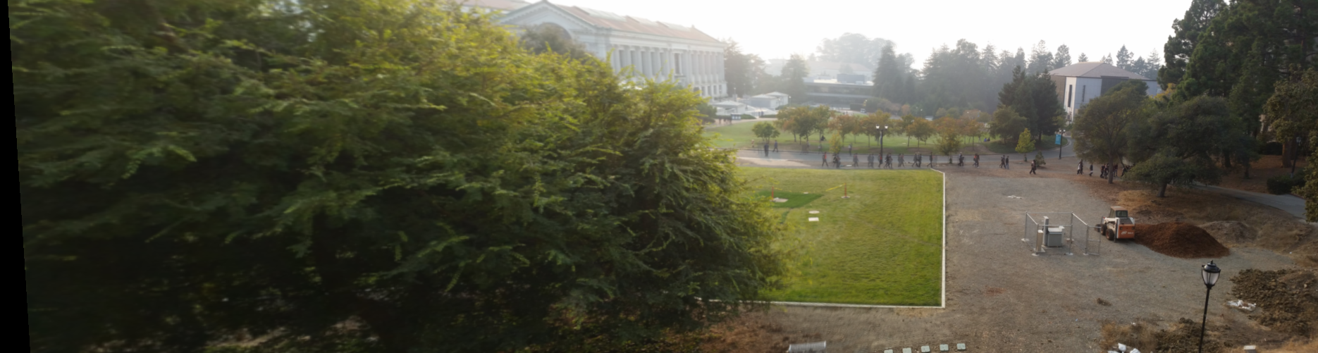 my favourite image mosaic result
|
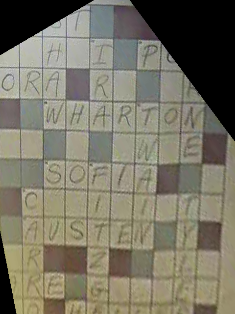
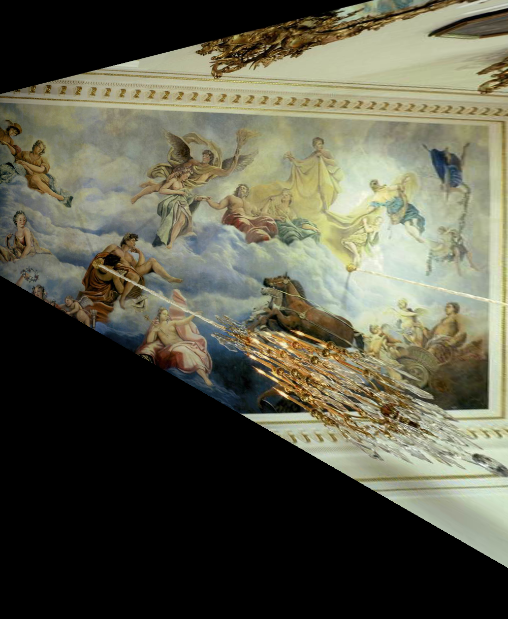
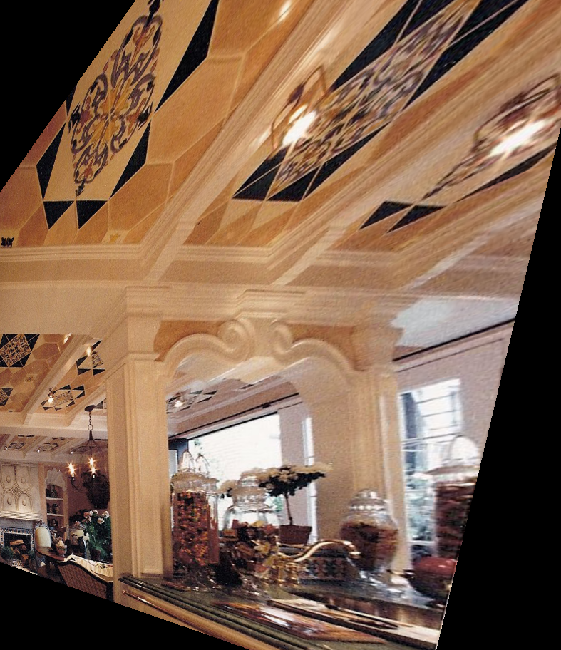
Through completing this part of the project, I consolidated my understanding of homographies, finally understood the pro's and con's between forward and inverse warping, forward warping is no good because not every pixel in the destination image will be filled! I learned that to accurately predict the size of a result image we can apply a forward warp to the corners of an image first. I think Image Rectification is actually what i personally find coolest about this project, in class we saw how we could see floors of paintings and that inspired me to do similar and look at cool ceilings! Finally I learned that picking points accurately and with a decent spread across the image is crucial to getting a good stitching. Smartly picking points is far more effective than blindly adding more, and I can't wait for part 2 where I'll write code such that I'll never have to pick points again.
Part 1: Shoot Images
Part 2: Image Rectification
Part 3: Blend Images into Mosaic
Part 2
Part 4: Detect Corner Features in an Image
The first part of automatic point picking is to detect Harris corners, code to detect Harris corners. For this entire process I will be using images I captured in Part 1 of Doe Library. Note that colors are slightly off due to the way cv2 saves images with different colour channels, final results are unaffected, and points are still clearly visible.
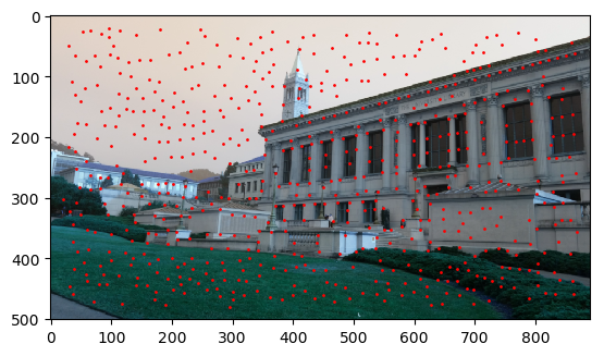 Image 1: Harris Corners
|
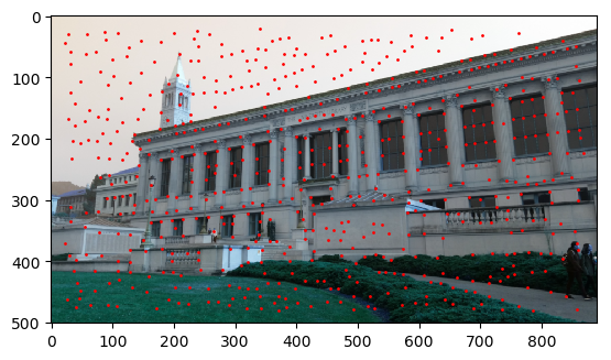 Image 2: Harris Corners
|
Once Harris corners are found, we notice that there are far too many, thus we use Adaptive Non-Maximal Suppression to reduce the number of points to the 500 "strongest" Harris corners in each image. This is done as per the equation in the paper, a constant of robustness of 0.9 was used as in the paper. Resulting points are shown below.
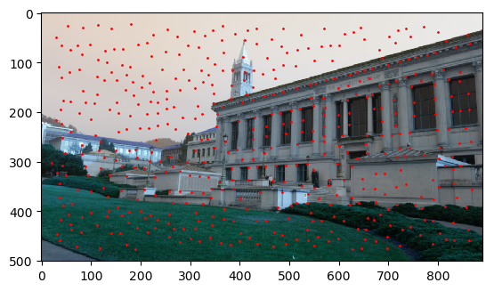 Image 1: 500 ANMS Points
|
 Image 2: 500 ANMS Points
|
Part 5: Extracting & Matching Features
The next step is to extract features for each points to try match points between image 1 and 2. Windows of 40x40 pixels were taken across the image, subsampled to 8x8, normalized, then flattened. These features were then matched to one another via distance comparison using the dist2 function given. The ratio between the top 2 matches were taken (1-NN / 2-NN) and if the ratio was below a certain threshold I chose to be 0.2, then the point was determined to be a good match. On average this would drop the number of resulting "matching point pairs" from 500 --> ~30.
 Image 1: Matched Points
|
 Image 2: Matched Points
|
Part 6: RANSAC
Finally, to ensure that no anomalous / invalid point matchings were made, I used the RANSAC method to randomly subsample 4 points from Image 1, compute a homography matrix from them, test the H matrix on all the points in Image 1, and count the number of points for which the homography is "valid" by an L2 norm comparison with corresponding points in Image 2 and a threshold I chose to be 0.3. This was repeated for 2000 iterations, and the largest set of inliers was used to compute a final homography matrix.
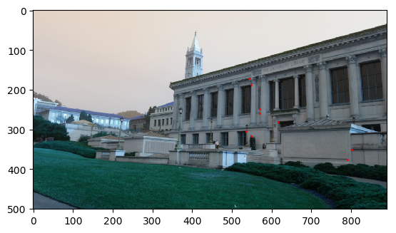 Image 1: Final Correspondances
|
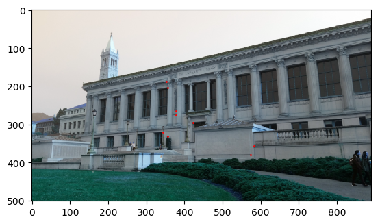 Image 2: Final Correspondances
|
Part 7: Final Auto-Mosaics & Comparison
Finally, with the automatically, computer-generated correspondance points the steps above determined, we repeat the procedure used in part 1 to generate homographies, warp, stitch and blend images together, to generate the results below. For comparison manual results from part 1 are also displayed below alongside automatic results as labeled.
Project Final Takeaways (Part 2)
I think automatic point detection is incredibly cool and powerful. Point selection in Part 1 was incredibly tedious, and also imprecise. As my results above show, computer generated points can achieve the same output results using less than half the points I manually picked. This project also improved my skills at reading techinical papers and translating them into functional code, a skill I am sure will be useful for my final project and other projects in the years to come.