Collin Chin's Programming Project #6B (part 2)
collin.chin@berkeley.edu
cs194-26-abx
Part 1
Recover Homographies
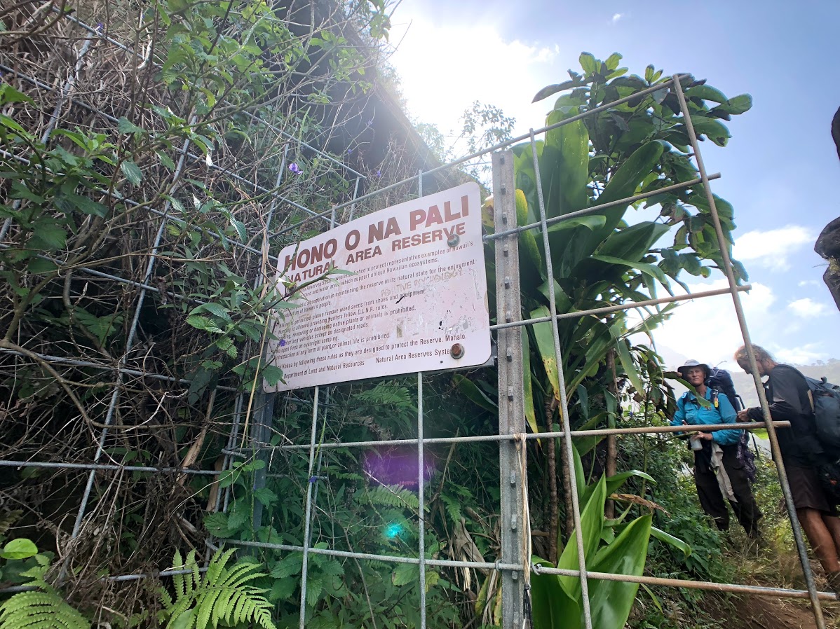
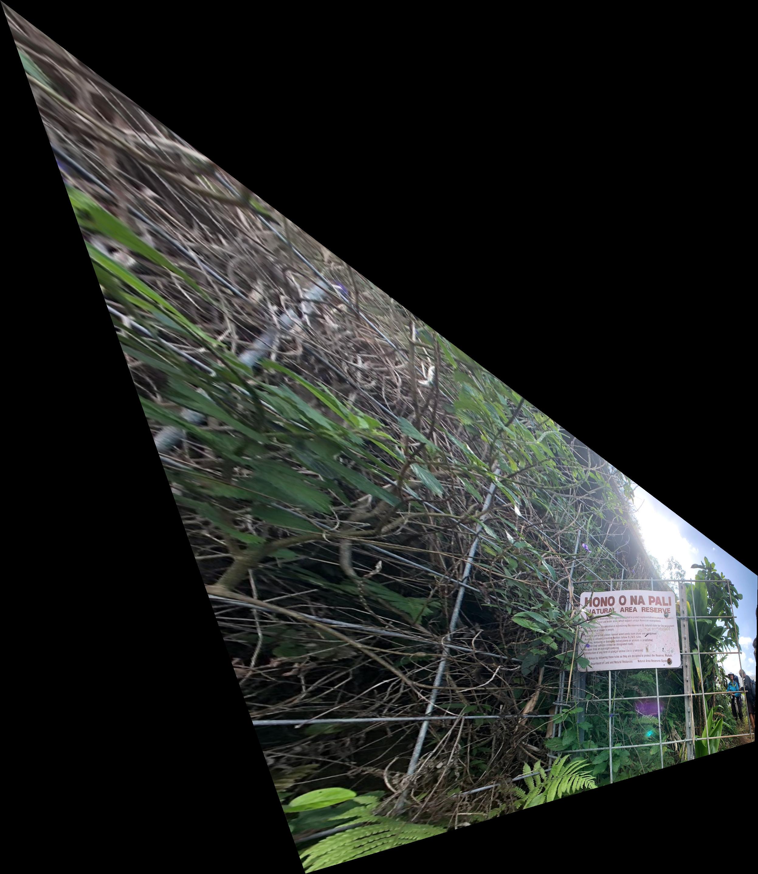
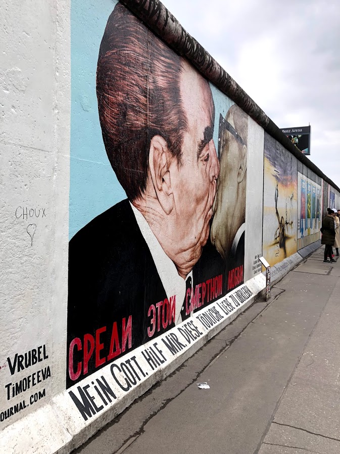
Given an image, we would like to reproject it so that it appears like the picture was taken from a different camera view. This problem can be expressed as finding a projective mapping H (homography) between two sets of points p and p' selected from the images with the same center of projection. We solve the equation p = Hp' using SVD and solving for H:3x3 with 8 degrees of freedom.
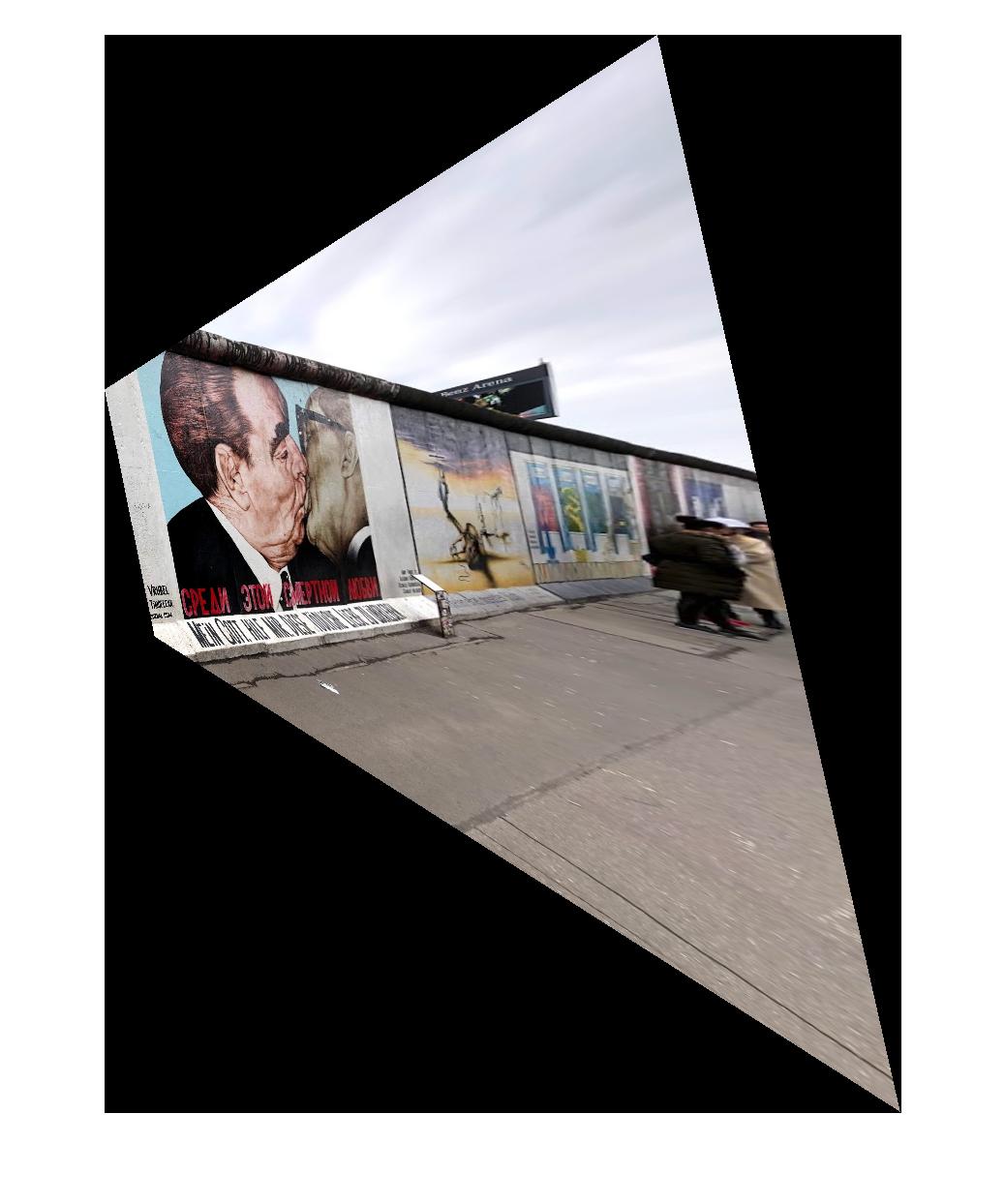
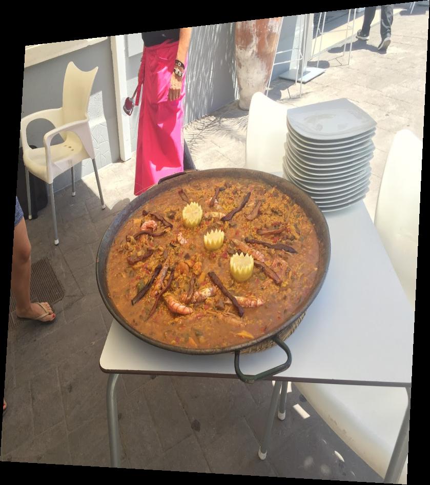
Warp Images
Using the homography matrix H from above, we apply the transformation to the original image and use interp2 to infer pixel values along uncertain spaces. The original sets of points in the previous part determine the bounding box for the resulting image. I noticed that results are better when the correspondence points p and p' cover a larger area of the image. Otherwise, the rectified image ends up with a lot of black unmapped pixels.
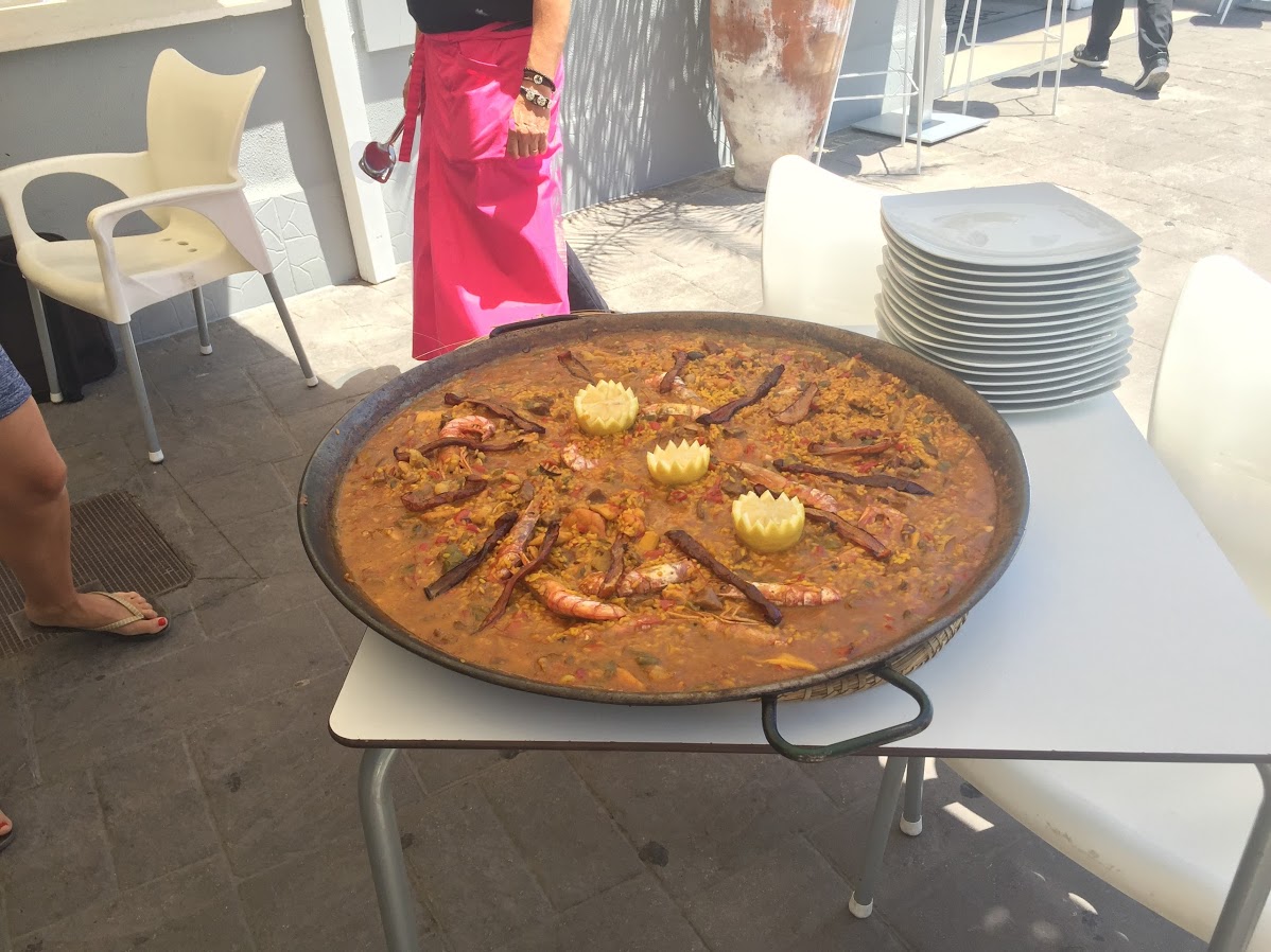
Image Mosaic
In this part we use weighted averaging to blend images taken from the left, right and center perspectives into one panorama. Six correspondence points between each image and the center designate the values to be computed for the homography. We define the final size of the mosaic and compute a stack of images to use for the mosaic. We use bwdist to linearly blend the images into one. Errors such as high frequency cutoff result from using this technique.
Part 2
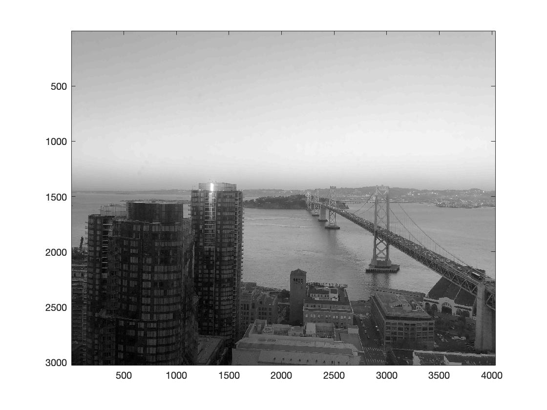
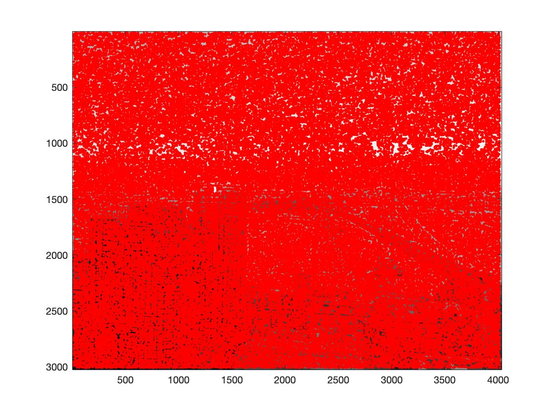
1. Detecting Corner Features
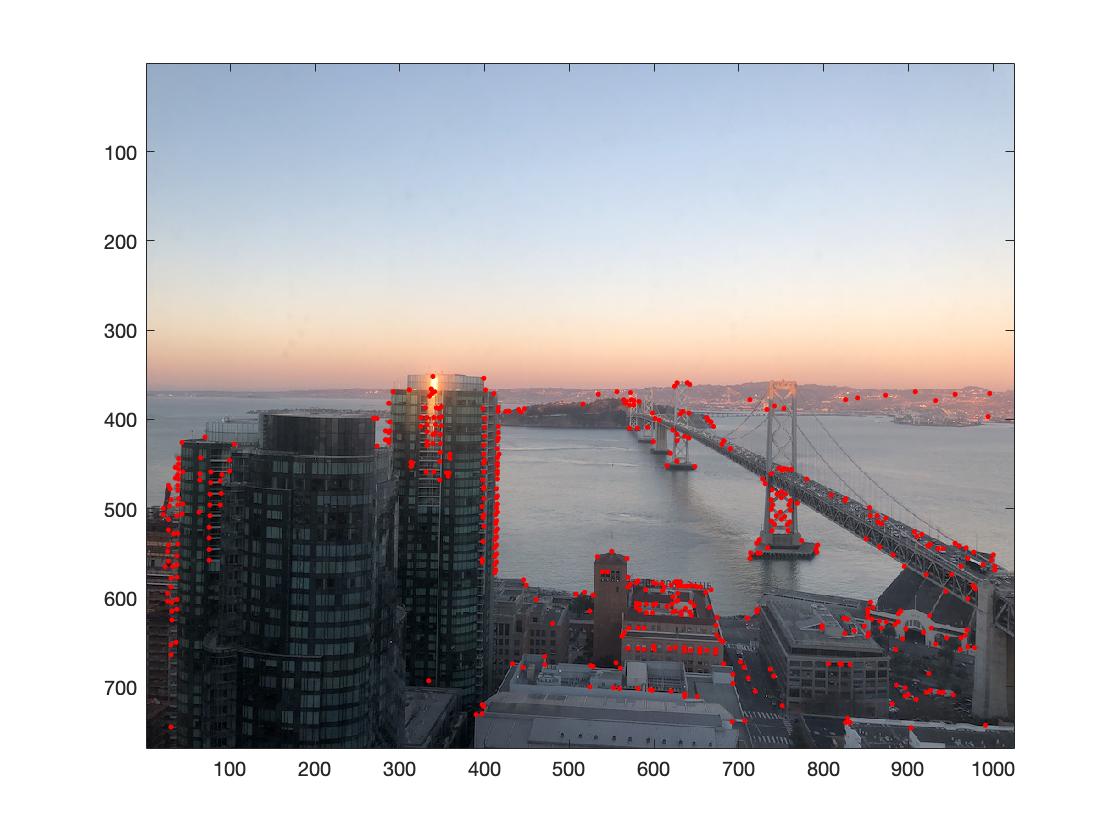
Our goal by step 5 is to automatically produce a mosaic using feature matching between three images. The first step is to identify points of interest that we can turn into features. The easiest point of interest to find in an image is a corner. We use professor Efros's implementation of a single-scale Harris Corner detector that looks at an input image(left) and identifies all corners(right, in-red). We can see that the top level of the pyramid sees a ton of corners. This will be resolved in the next part.
2. Extracting a Feature Descriptor
To restrict the maximum number of interest points extracted from each image, while keeping them spatially well distributed over the image, we use Adaptive Non-Maximal Suppression. This method computes a corner strength function and retains corners that are a maximum in a neighbourhood of a specified pixel radius.
3. Matching Feature Descriptors
In this section, we define local feature vectors for each image by sampling and normalizing an 8x8 patch of pixels around the interest point.
4. Compute Homorgraphy using RANSAC
Next, we match the feature vectors from the previous part by using the RANSAC algorithm:
1. selects N data items at random
2. estimates parameter x
3. finds how many data items (of M) fit the model with parameter vector x within a user given tolerance. Call this K.
4. if K is big enough, accept fit and exit with success.
5. repeat 1..4 L times
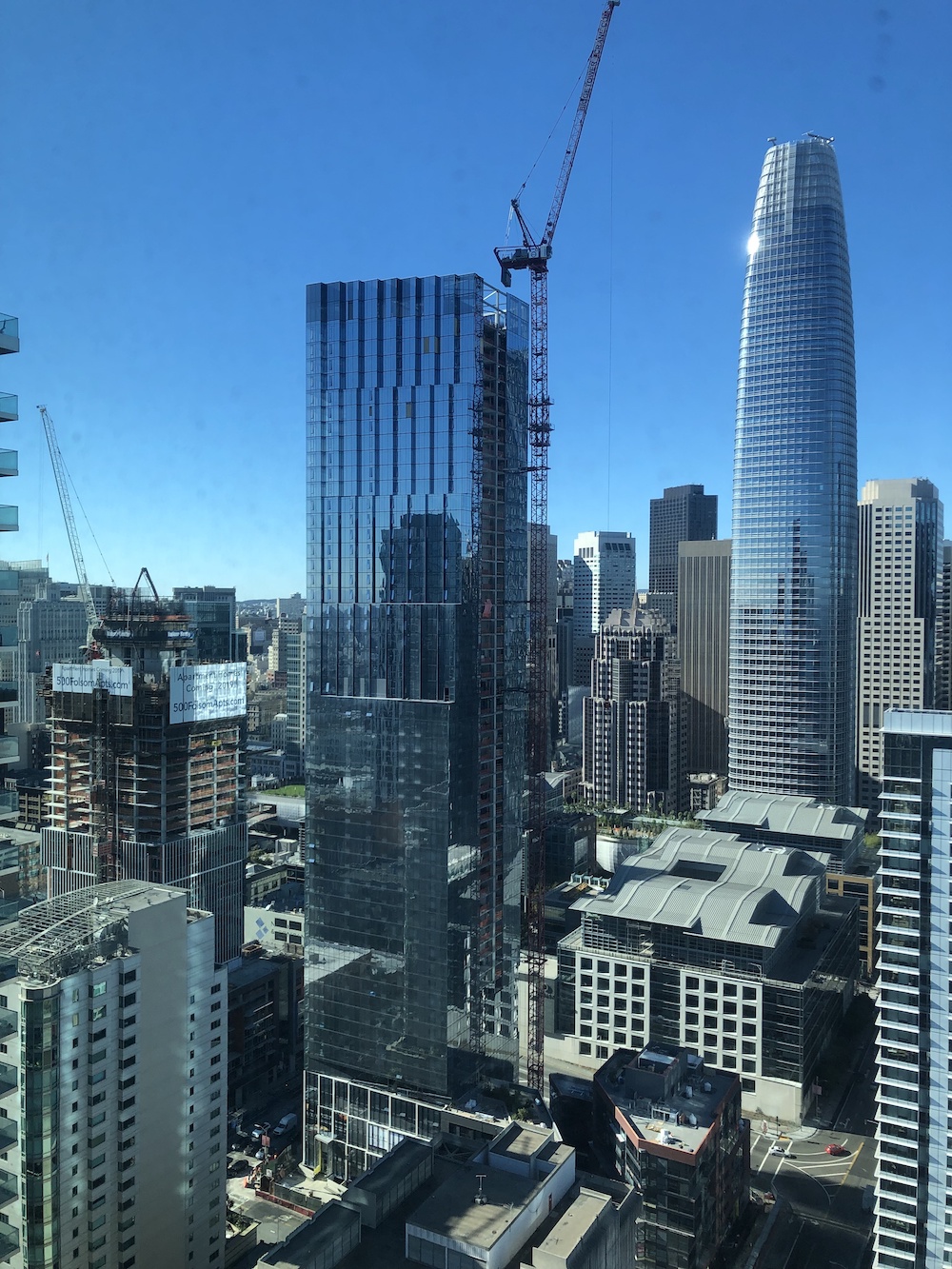
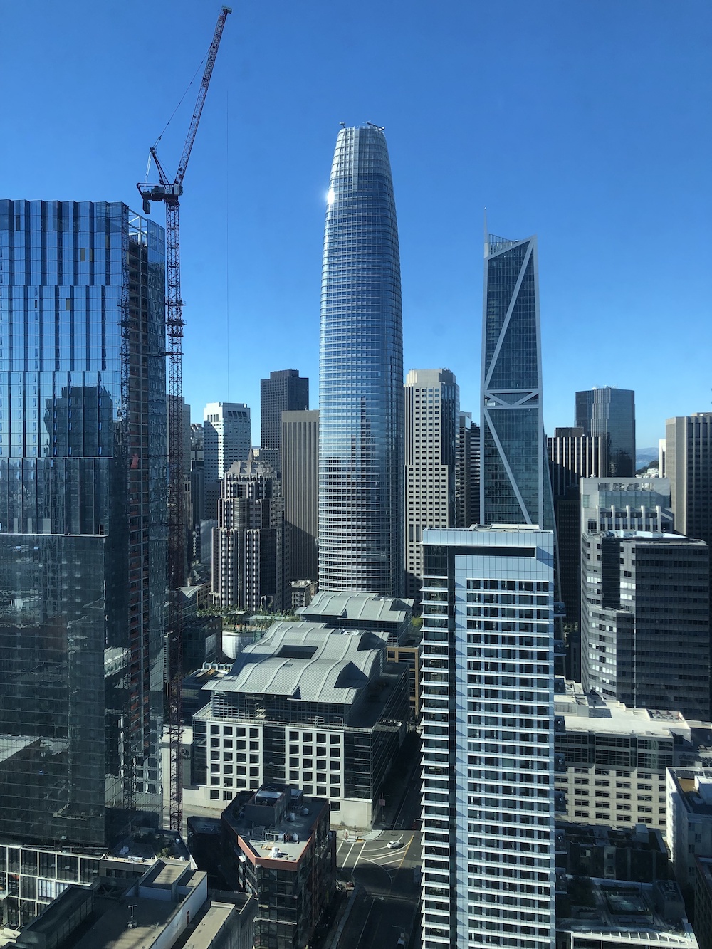
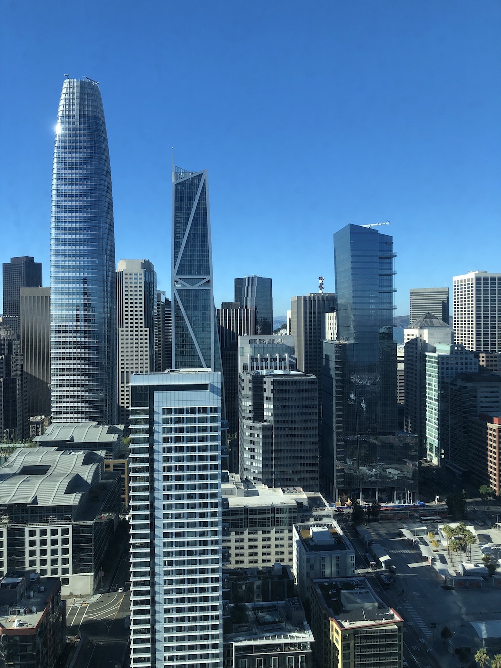
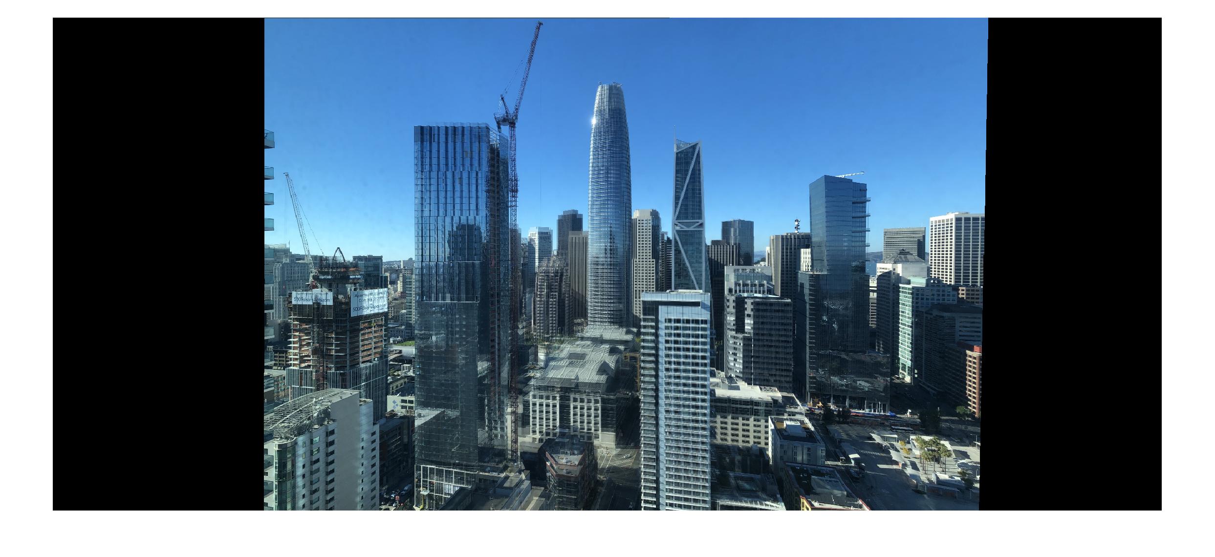
5. Mosaics
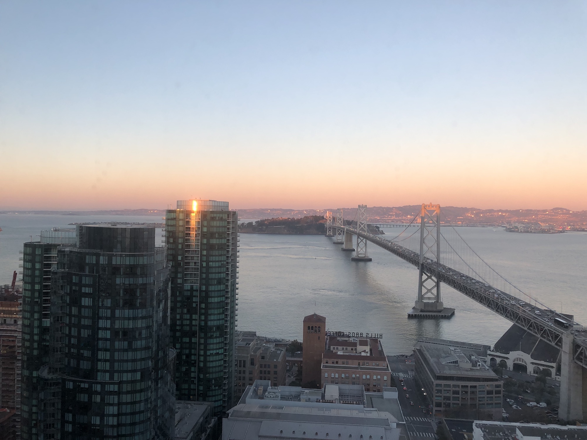
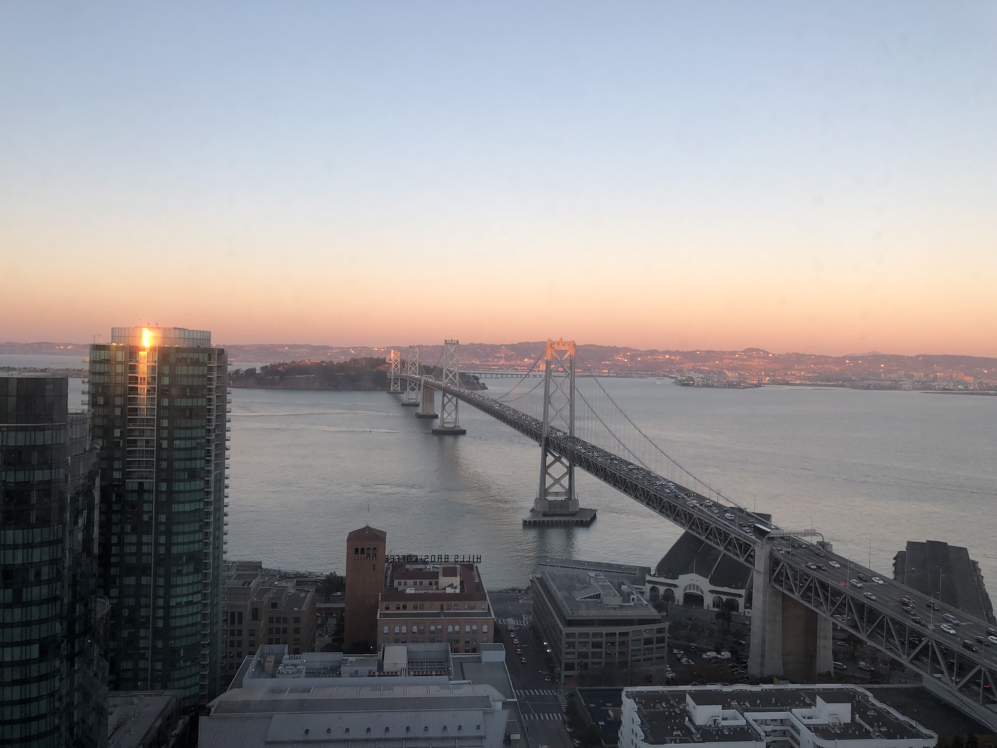
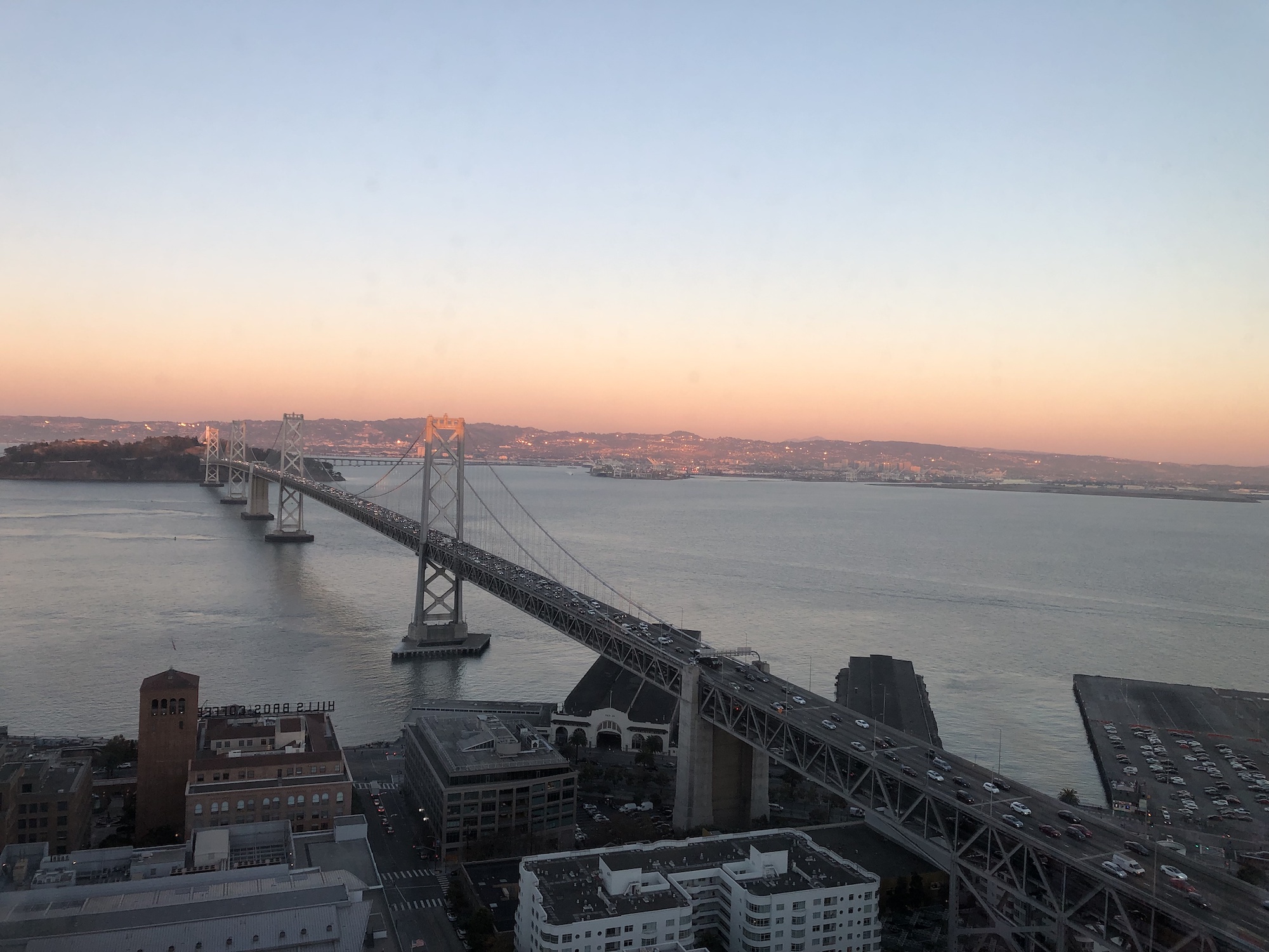
Here are the final results for the bay bridge panorama.
The first three images are the originals. The next three images show the points of interest selected by ANMS. The seventh image is the result of Project 6A - Manual feature selection. The last image is mosaic formed by the entire feature matching for autostitching project.
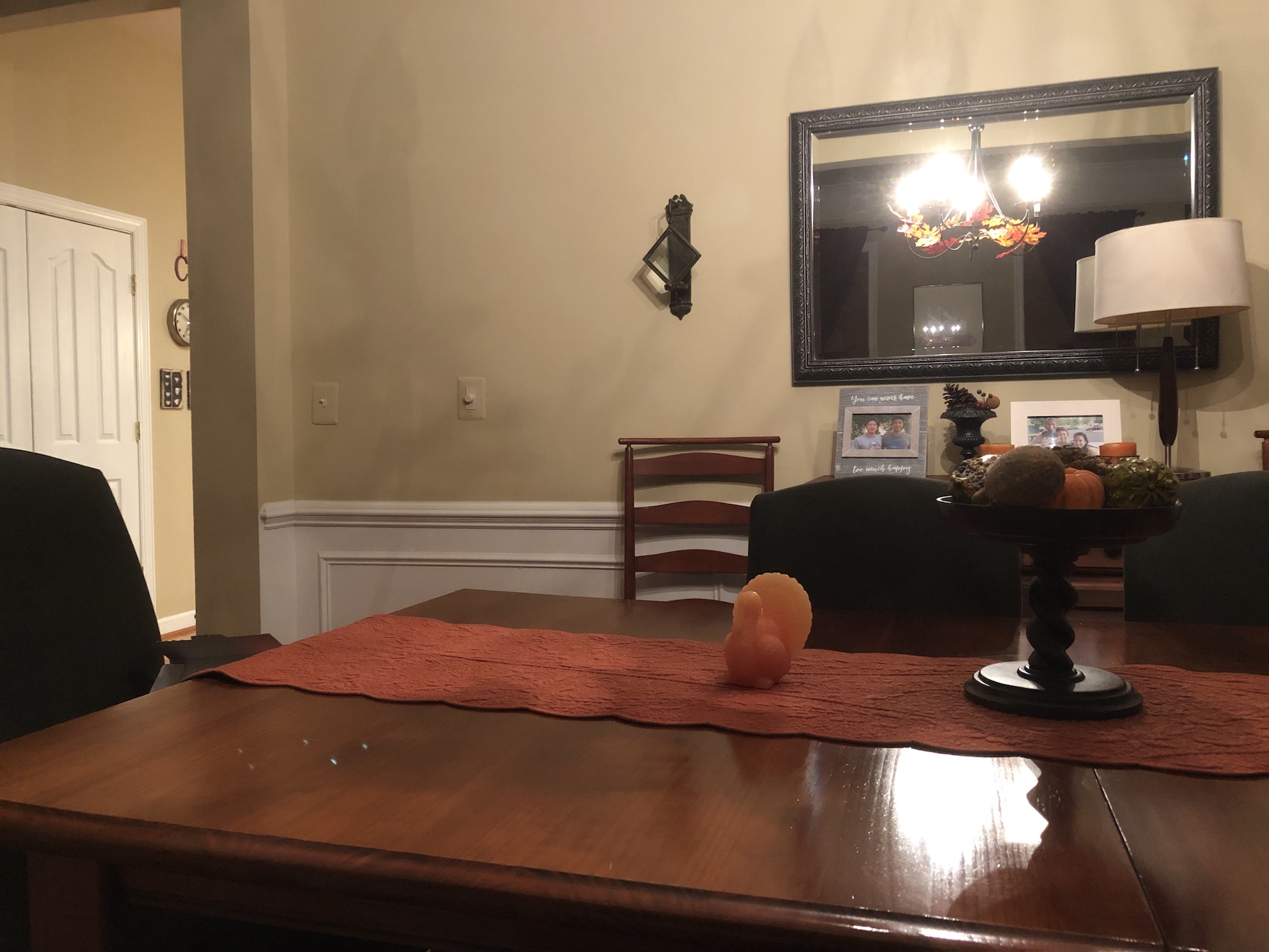
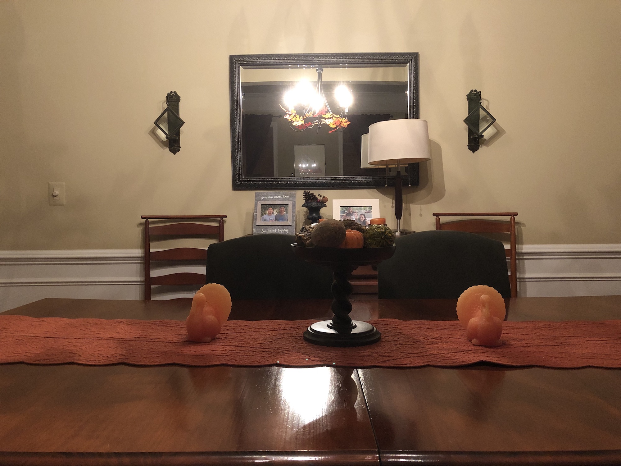
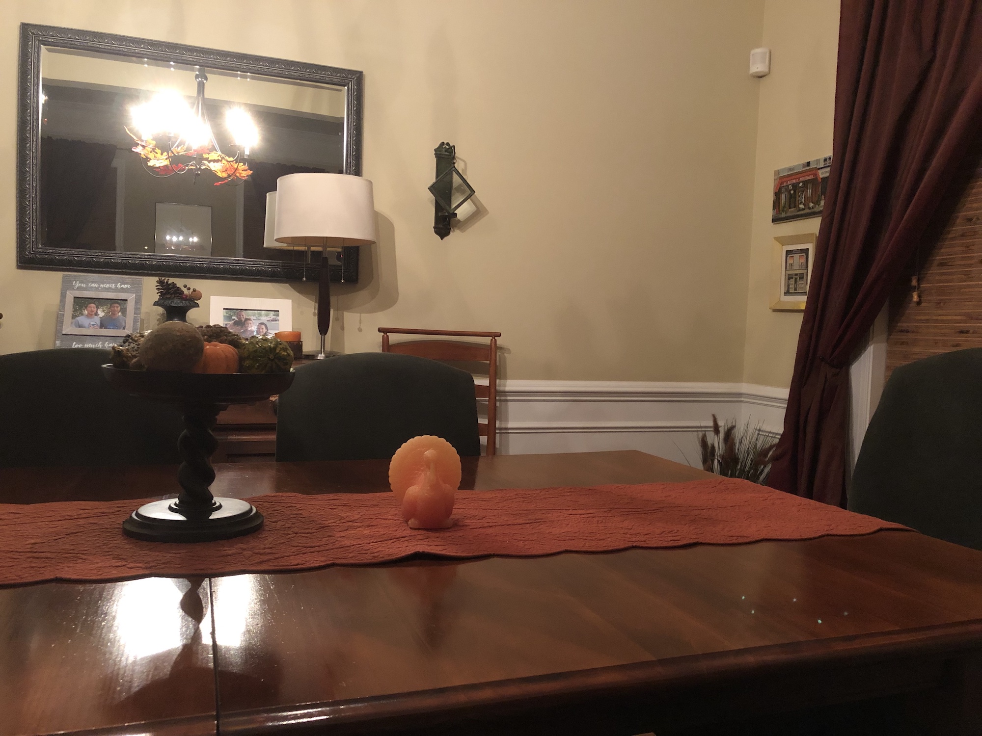
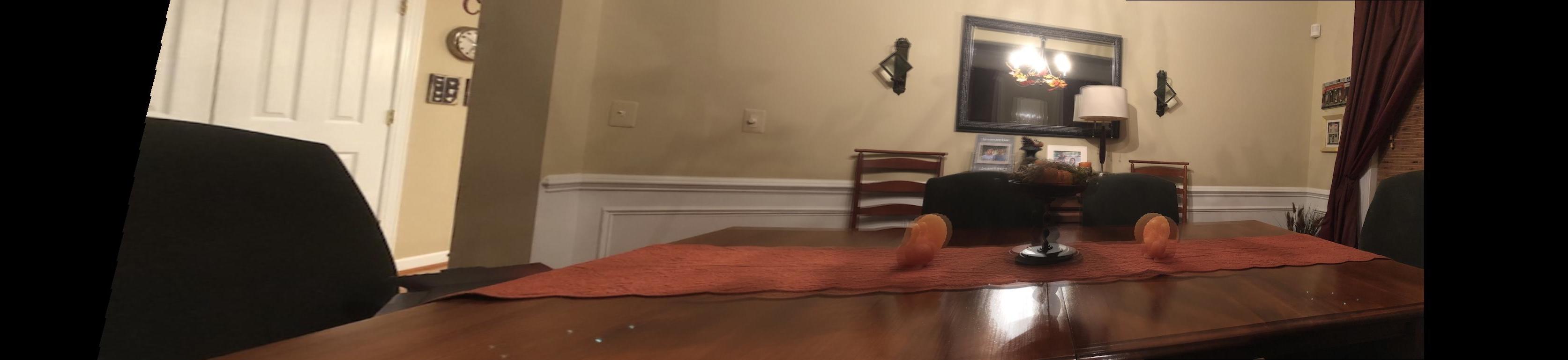
Dining Room
The first three images are the originals. The fourth image is the result of Project 6A - Manual feature selection. The last image is mosaic formed by the entire feature matching for autostitching project.
Living Room
The first three images are the originals. The fourth image is the result of Project 6A - Manual feature selection. The last image is mosaic formed by the entire feature matching for autostitching project.
Learning
This was by far the most comprehensive project in the class. What I found most interesting was how random data point selection could be used to form extremely accurate panoramas.