For this project, we calculated homographies after defining correspondences between two photographs with projective (perspective) transformations, meaning the camera didn't translate between taking the photos. Using the computed homographies, we can then "rectify" an image and create image mosaics.
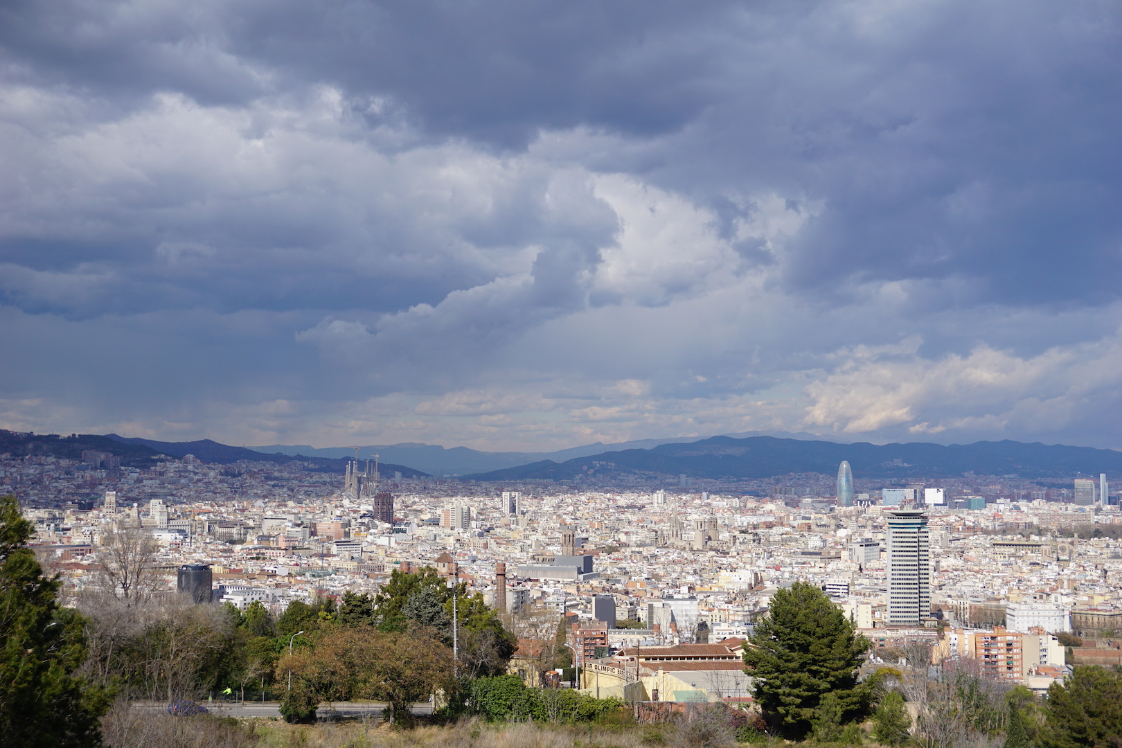
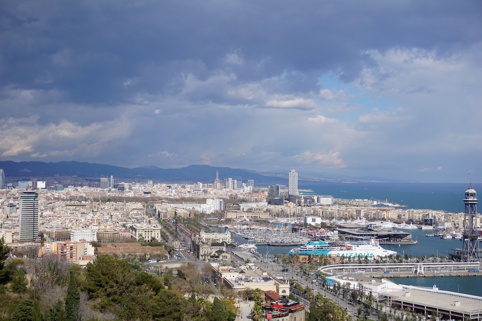
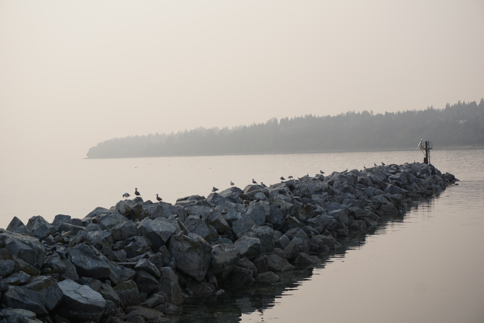
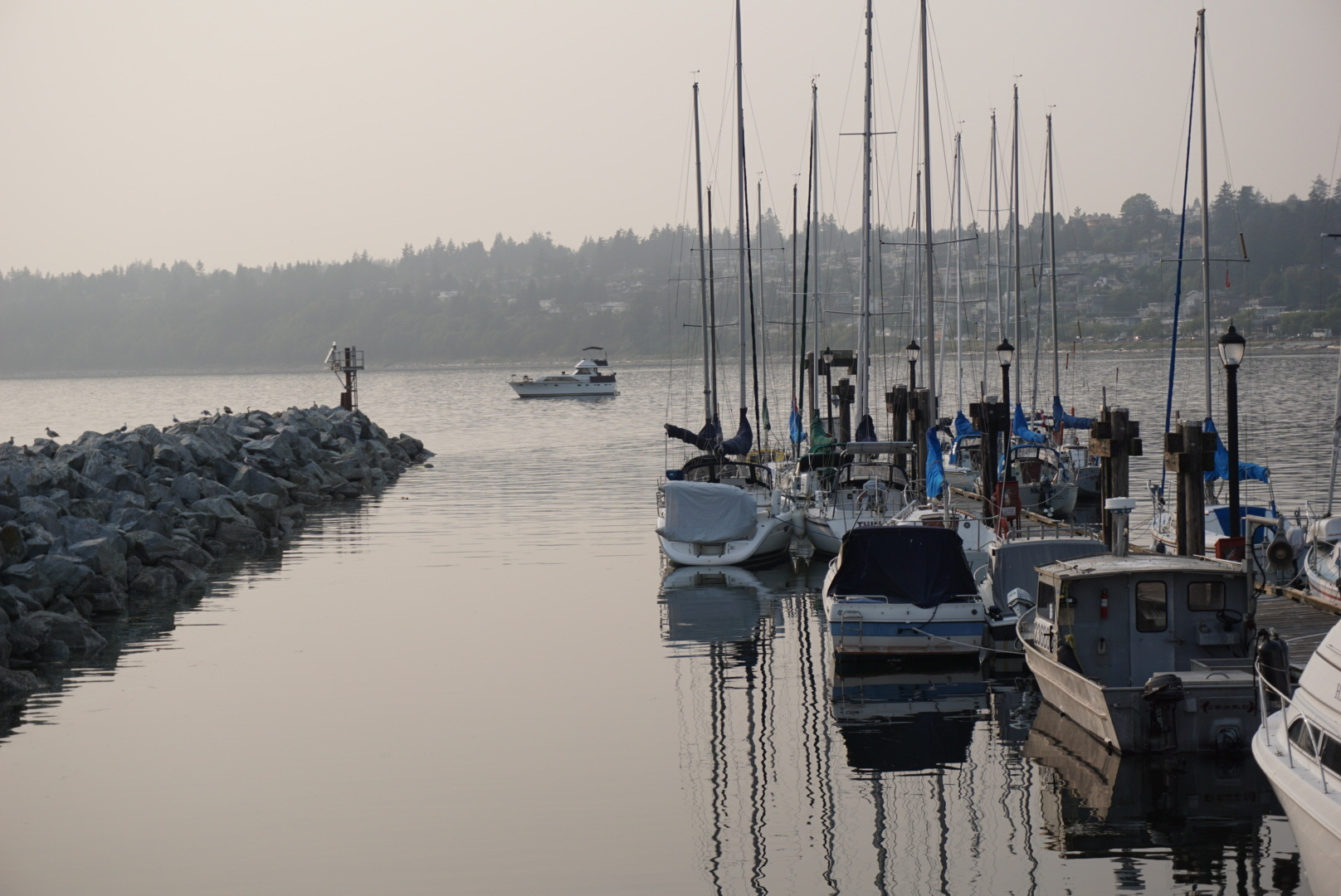
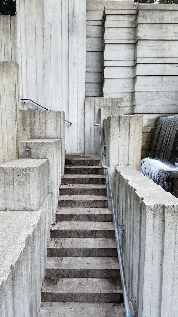
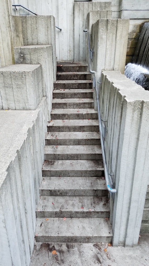
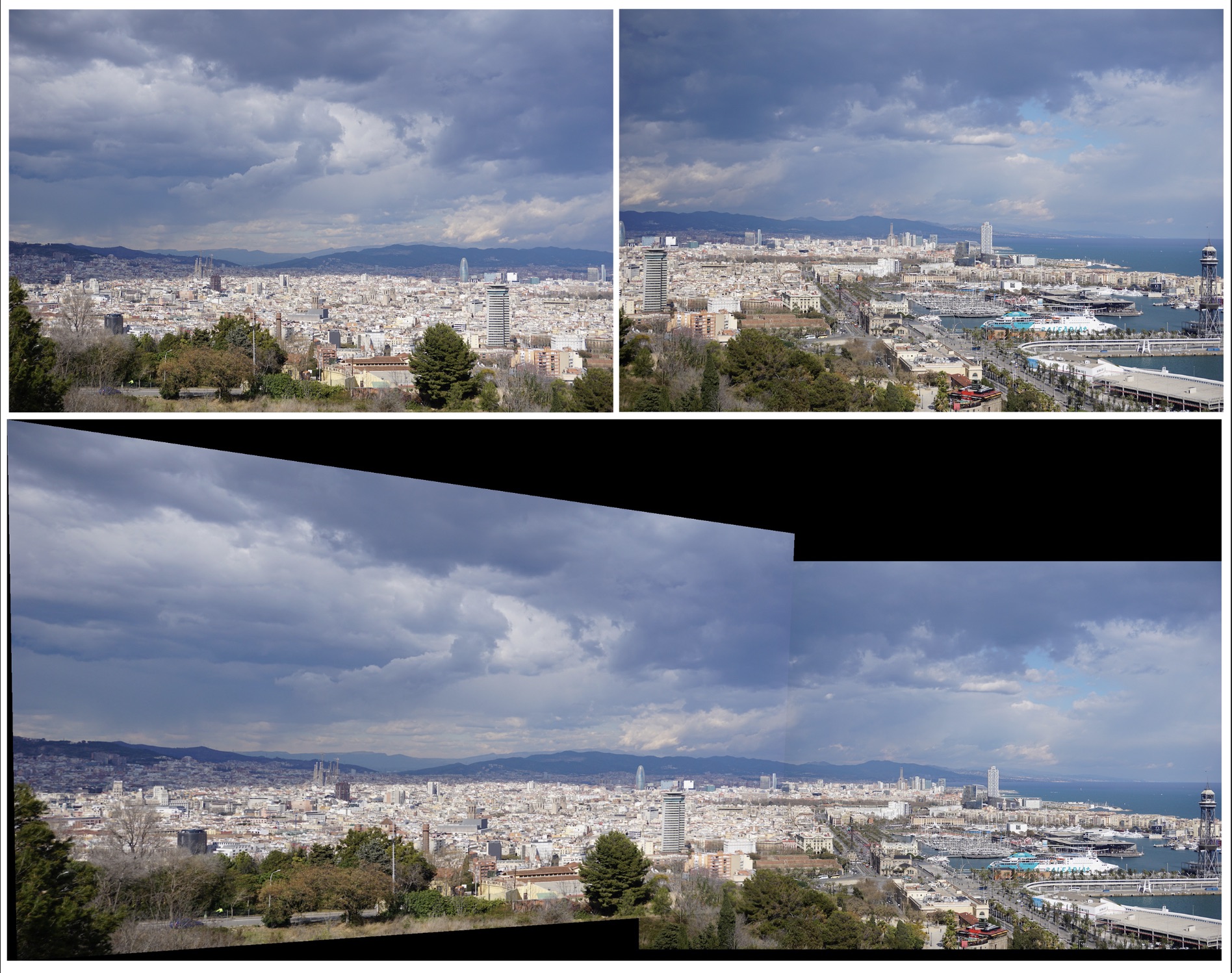
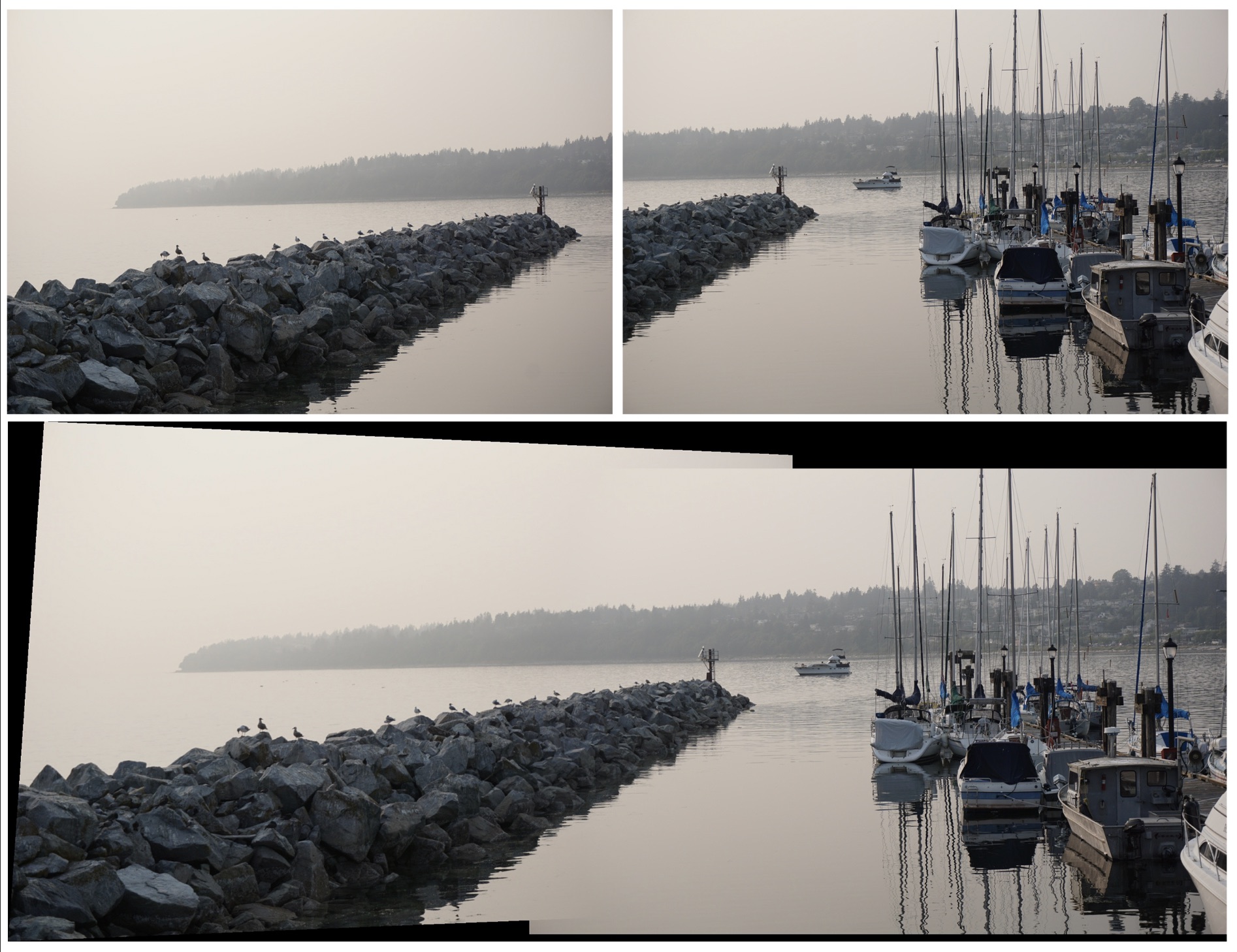
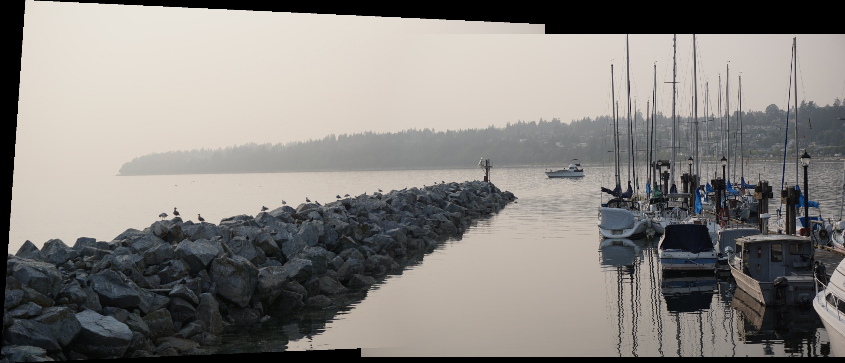
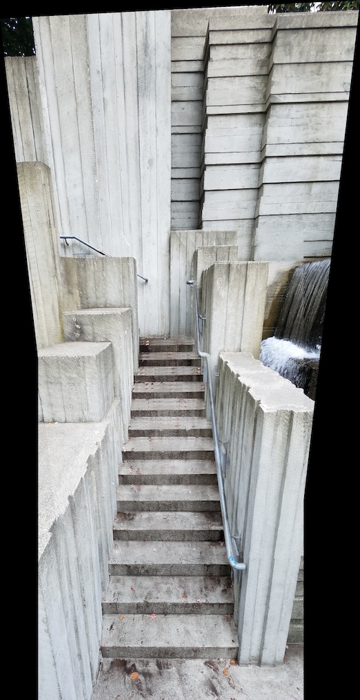
The photos I chose to create a mosaic were taken prior to this class during my trips to Barcelona in 2016 and Seattle/Canada this past August, and they happened to have a lot of overlap!
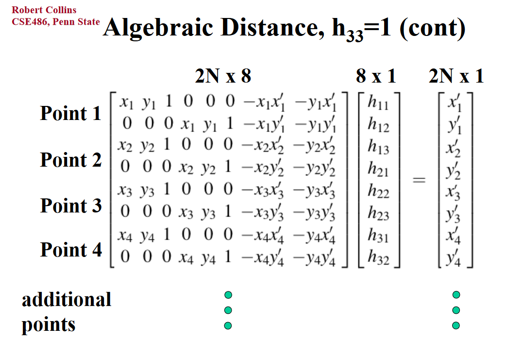
In order to warp our images, we need to recover the homography matrix that provides the transformation between the pair of images. I constructed a matrix of the following form, where (xi,yi) and (xi',yi') are pairs of corresponding points of the two images. We then solve for the 8 unknowns and append a 1 to the end since the lower right corner is the scaling factor. This gives us the 3x3 homography matrix, which we use in the following sections.
Now that we have the homography matrix, we can warp one image to the perspective of another. My warp function is modified
from the warp function I implemented in Project 4 where I again used inverse warping.
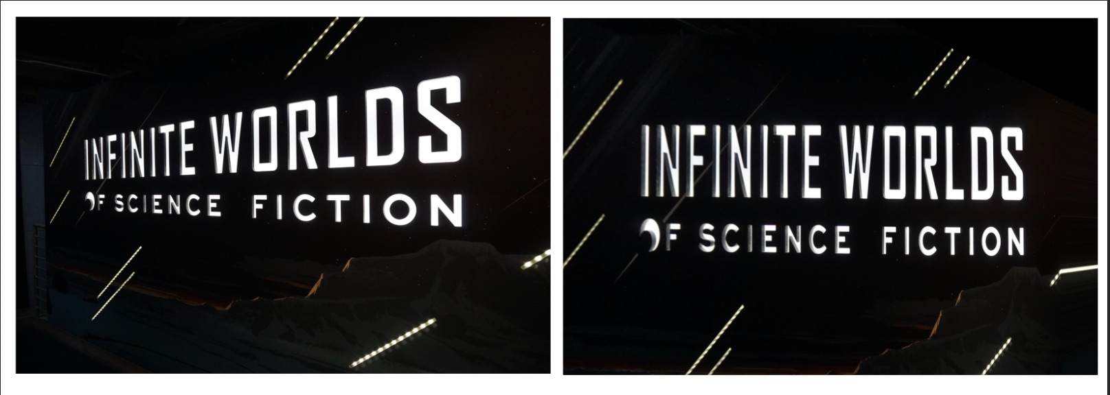
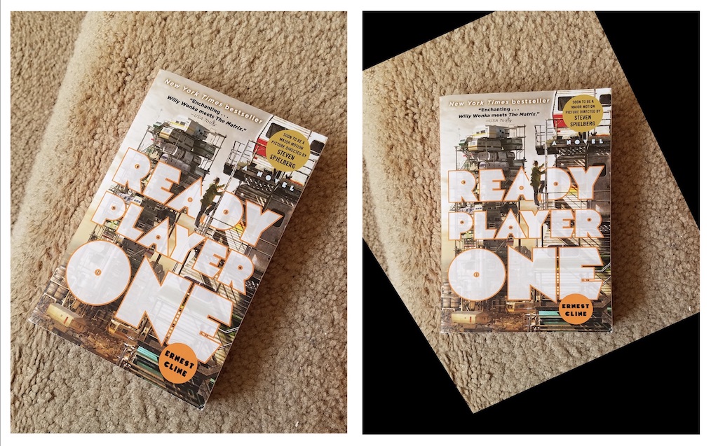
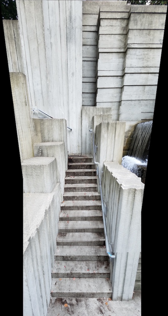
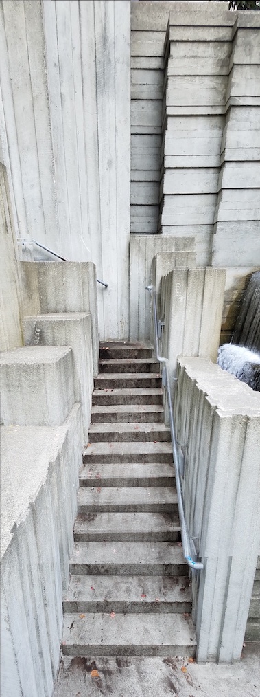
First, I started small to ensure that I have computed the correct homography matrix and implemented the right warp function. I tested
photos where the objects were taken at a perspective, and then applied my warp function so that the plane is now frontal-planar
(the image is flattened as if staring straight-on).
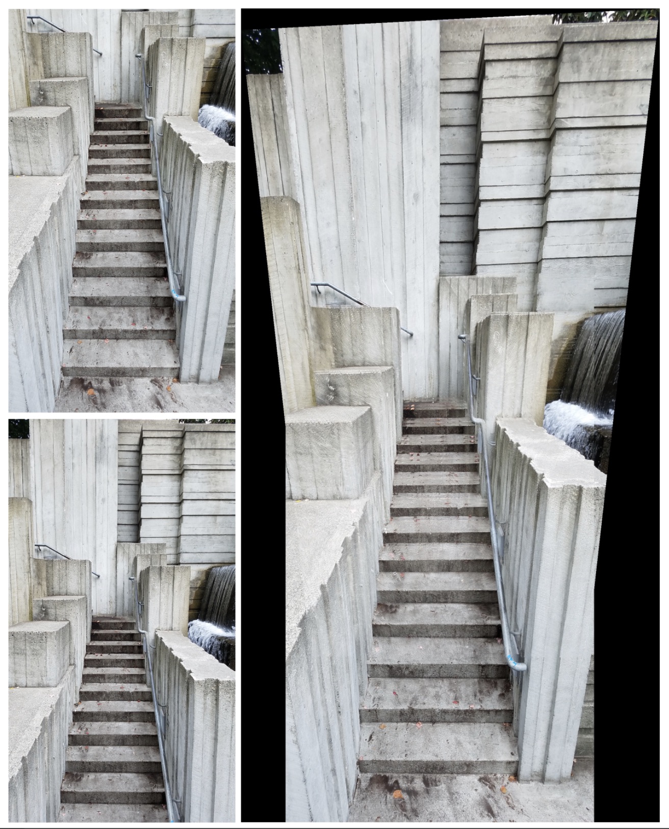
Here I warped the left image to the perspective of the right image, aligned the warped left image result with the right image using the offset computed when warping the left image, and then blended them together by taking the element-wise maximum using np.maximum.
The second part of this project aimed to automatically stitch two photos together to create a mosaic by implementing the steps laid out in the research paper, “Multi-Image Matching using Multi-Scale Oriented Patches” by Brown et al.
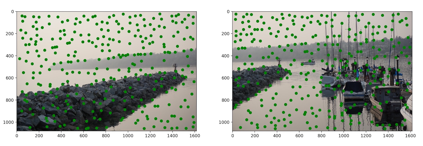
The first step was to detect corner features, which we found by using the Harris Point Detector in the provided starter code.
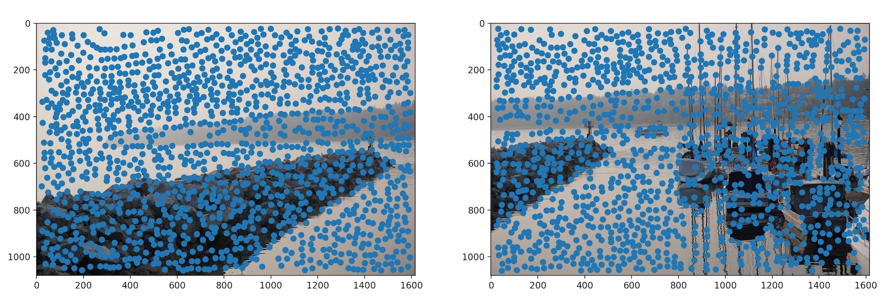
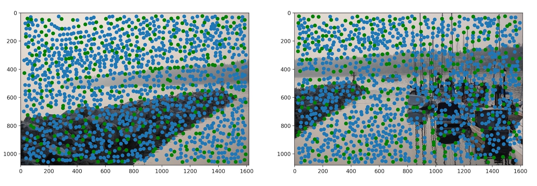
The Harris Point Detector outputs way too many points, so next we need to reduce these points such that they are uniformly distributed across the image. We can do this by implementing Adaptive Non-Maximal Suppression, which selects points that have a large distance between itself and its nearest neighbor with a high h value. We use the following formula:
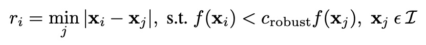
where xi is the current point we're looking at and xj is one of the other points. If the h value of xi is less than xj's h value multiplied by a constant c, which is defined to be 0.9, then we compute the SSD between xi and xj and record their distance. After finding the distance between xi and all other xj's that satisfy the constraint, we then find the minimum distance and map that to xi. Finally, we select the top 300 points with the largest distances.
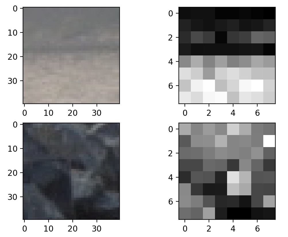
Now we must extract a feature descriptor for each feature point in order to match it with a point in another image.
I did this by taking a sample patch of 40x40 pixels around each point and normalizing the patch by subtracting the mean
then dividing by the standard deviation. I then resized the sample patch to 8x8 pixels using skimage.transform.resize
and mapped each patch to the point in a dictionary for easy access.
Here are the 8x8 patches for two randomly selected points:
To match the feature descriptors, I iterated through each point, p1, in the first image and computed the SSD between p1's patch and every patch in the second image, mapping the distance to point p2 in another dictionary. I sorted the distance from least to greatest, and took the first and second nearest neighbors, NN1 and NN2. If NN1/NN2 is less than a threshold (I chose the threshold to be 0.65), then it's a match!
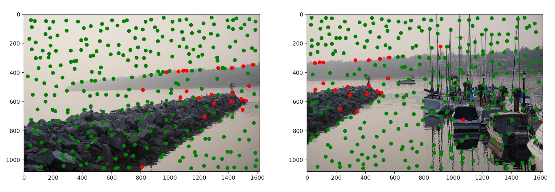
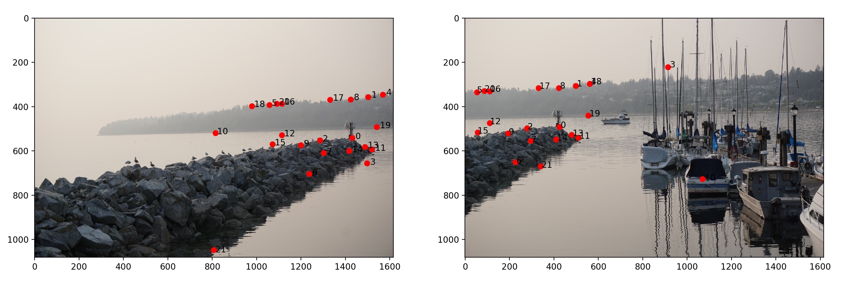
However, not all points matched correctly. For example, points 3, 10, 18, and 21 are incorrect matches. Now we must figure out how to identify and subsequently exclude these incorrect pairs.
The solution is to use the RANSAC in order to find and exclude the mismatched points. In 10,000 iterations, I randomly chose 4 pairs of matched features and computed a homography for these 8 points. Then I passed all of image1's points through the homography matrix and computed the SSD between the image1's warped points and image2's points. Using dictionaries, I mapped the pairs of points to the distance and only kept the pairs where the distance is less than 20. The number of inliers is the length of the dictionary. At the end of 10,000 iterations, I end up with a set of points that is considered to be the most inliers.
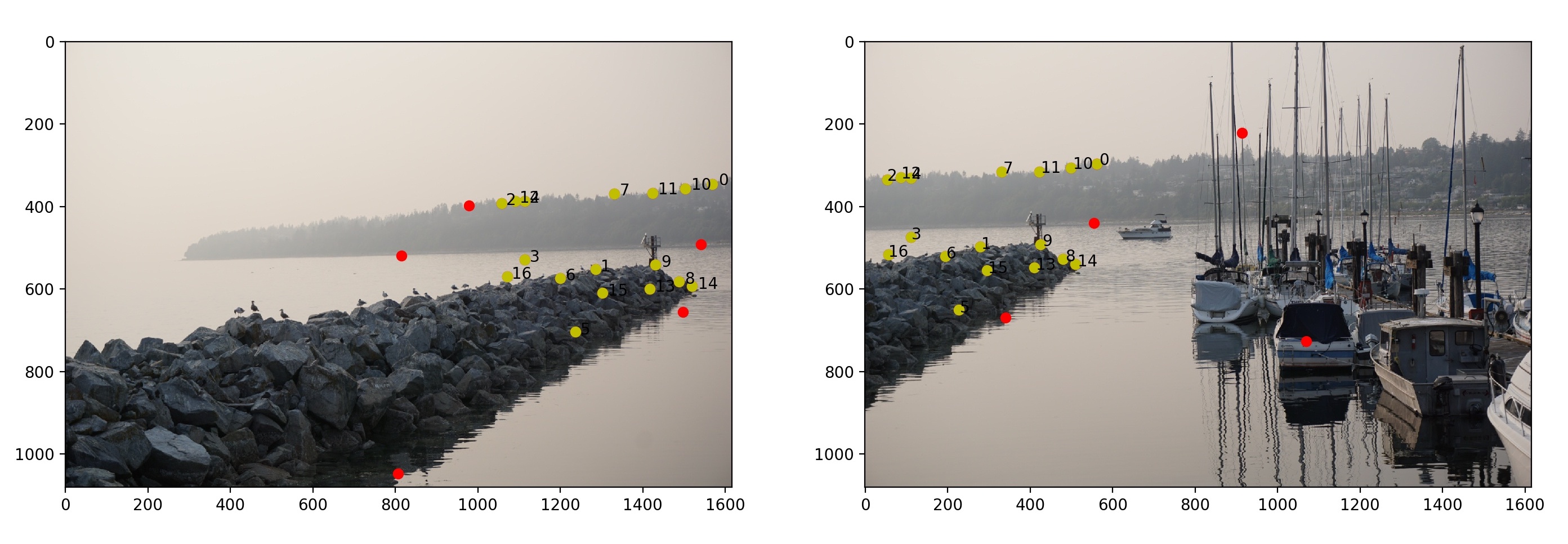
Finally, now that we have a set of correspondences from two images, I sent the two sets of points through the code I implemented in Part 1. These are the results:
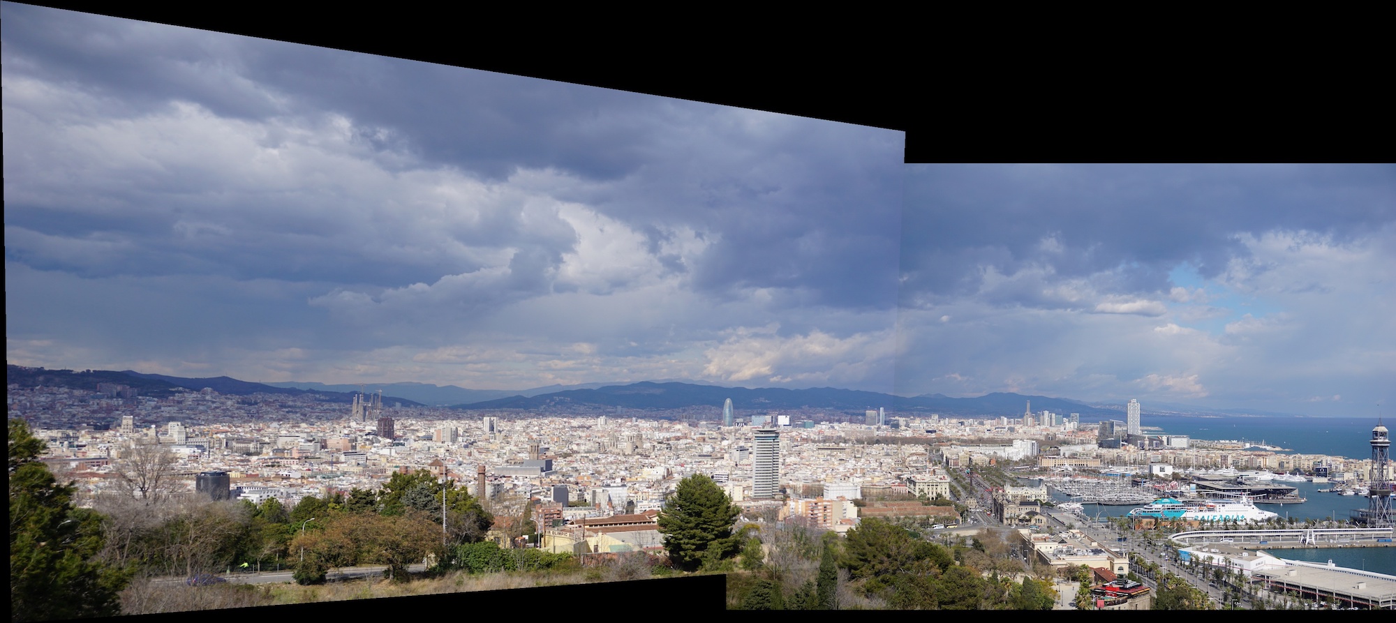
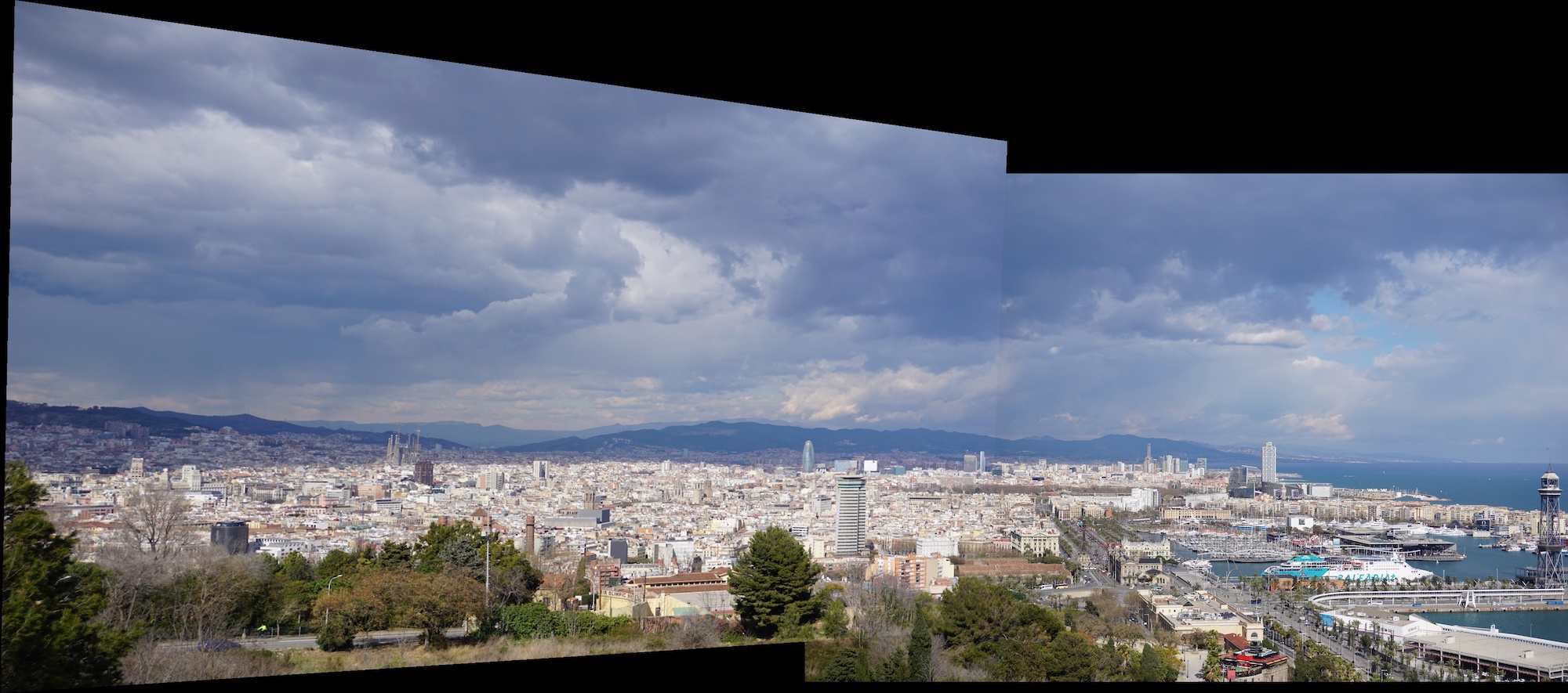
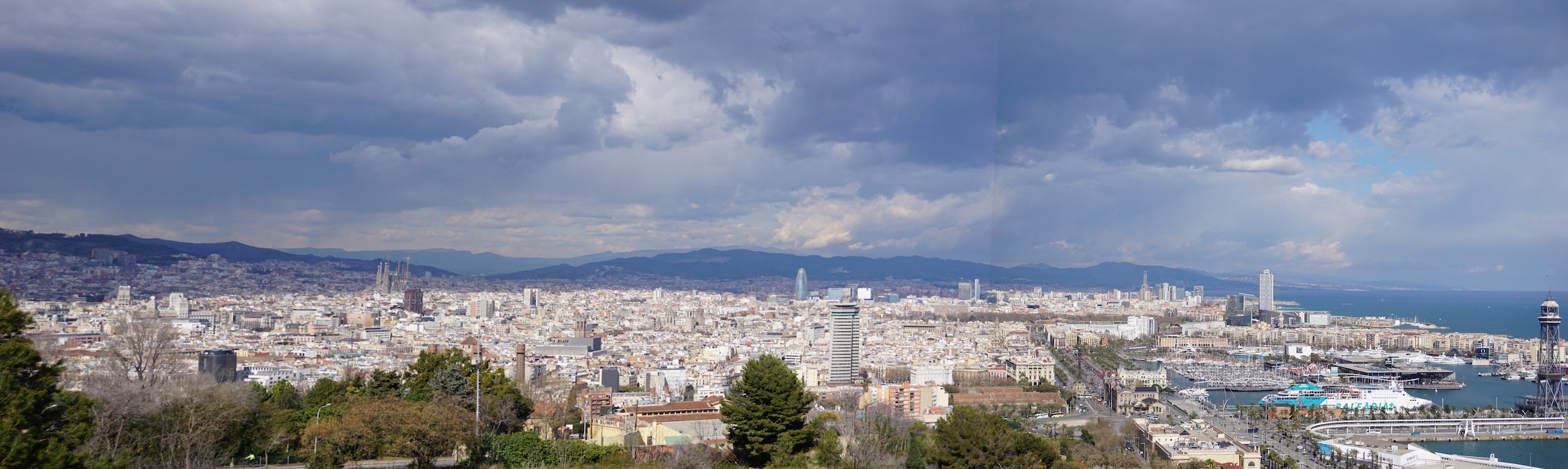

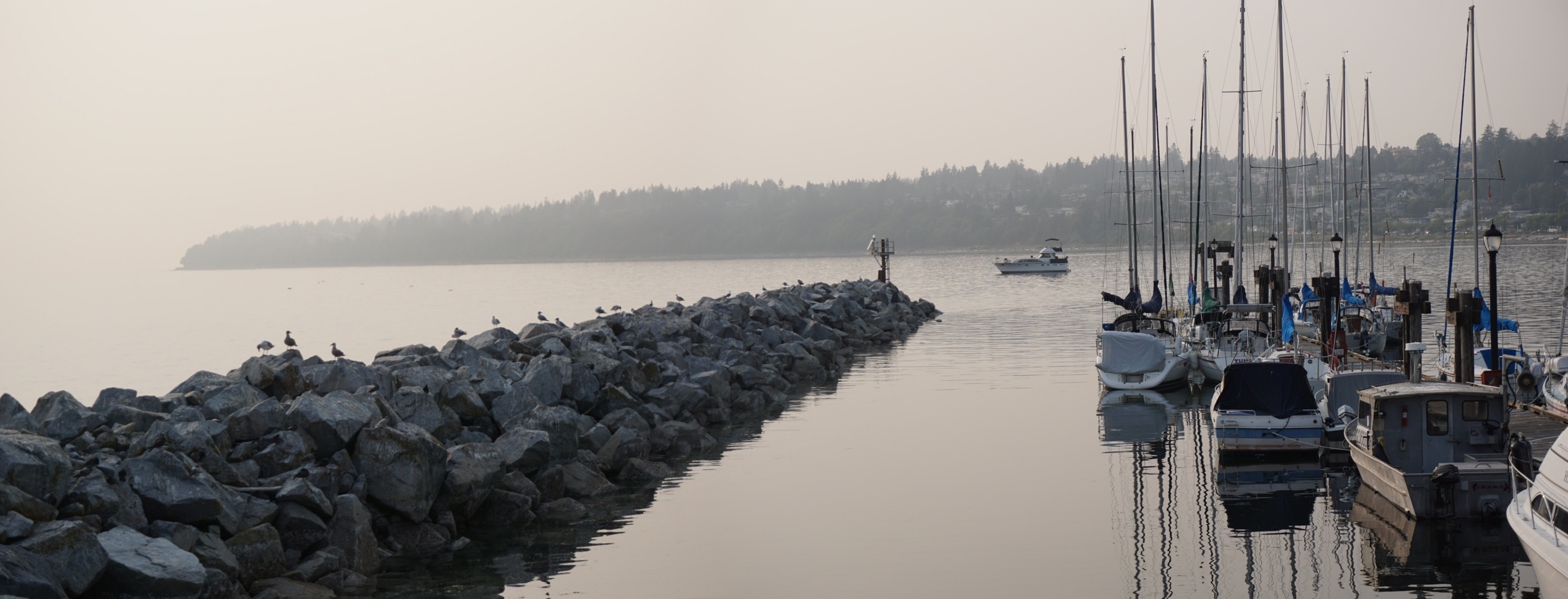
My manually vs. automatically stiched mosaics seemed to be about the same! Most likely because in the manual implementation, I chose 21 points that were uniformally distributed across the overlapping region. But it's great that I won't have to meticulously choose 21 points to create a panorama now with automatic stitching!
I learned a lot through this project, which has taught me so much about homographies and altering perspectives. It was
also great to use what I have learned and coded in previous projects and apply them here. In Part 2, it was interesting
studying (and fun implementing) the steps that is needed to create a panorama image. Dictionaries were my friends in Part 2,
and I learned a lot more about Python dictionaries and discovered some fun indexing tricks you can do with them.
I had a bug that continued since Part 1 where my images wouldn't align correctly. The resulting mosaic would be off by less than 20 pixels
in either direction, and I could not for the life of me figure out what was wrong. That is, until I started plotting points using matplotlib.pyplot
at various locations in my code. I was able to effectively troubleshoot by plotting points, and I learned more about how to plot points using
matplotlib.
The coolest part for me was that I was able to take photos I've taken months or even years ago
and either warp the image so that the object is now frontal-planar or take two photos and create a panorama after-the-fact.