To make image mosaics, we first need to find a homography H that maps one image to another. We do this by finding at least 8 pairs or correspondences between two images, p and p’, like below:
With these correspondences, we can set up a linear system of equations with the following form:
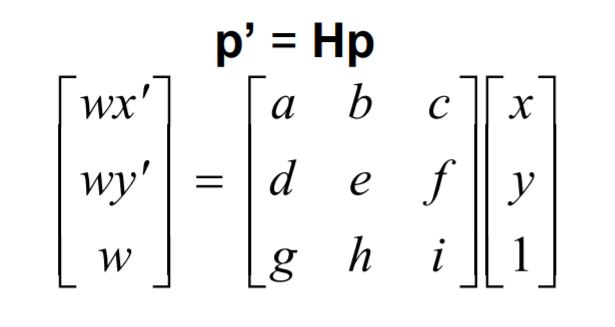
We can set i=1 because we only need a perspective transform, however, because we don't know w, we need to expand and rearrange some of the terms of our system. For each pair of points i in p and p', we have:
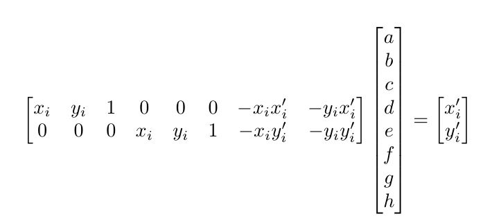
We can set up our A matrix and b vector as such to include all pairs of points, and use a least squares solver to recover the homography.
After writing functions that compute a homography between two images using a list of at least 4 correspondences, we can rectify an image by selecting 4 corners of a feature we know is a rectangle, and compute a homography between these points and some scaling of the unit square (or rectangle.) Then we find the inverse of this homography and use it implement an inverse warp between the original image and the rectified square:
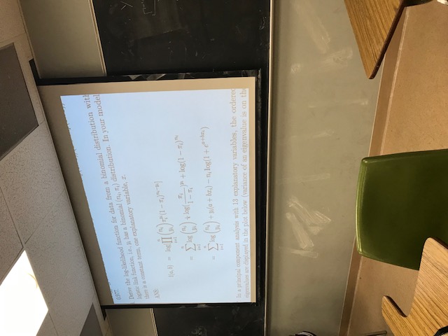
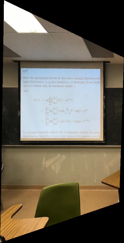
First I rectify a picture I randomly found on my phone taken during a discussion section:
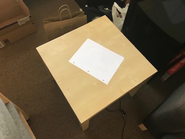
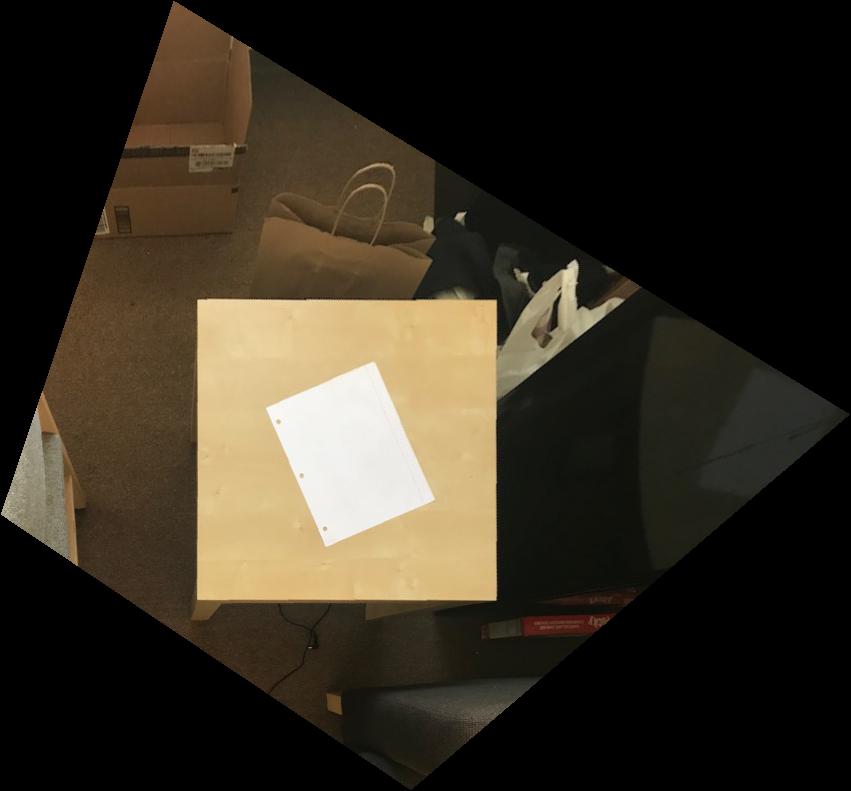
And then I rectify a square table with a piece of paper on it:
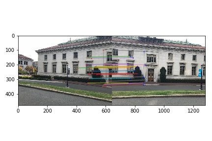
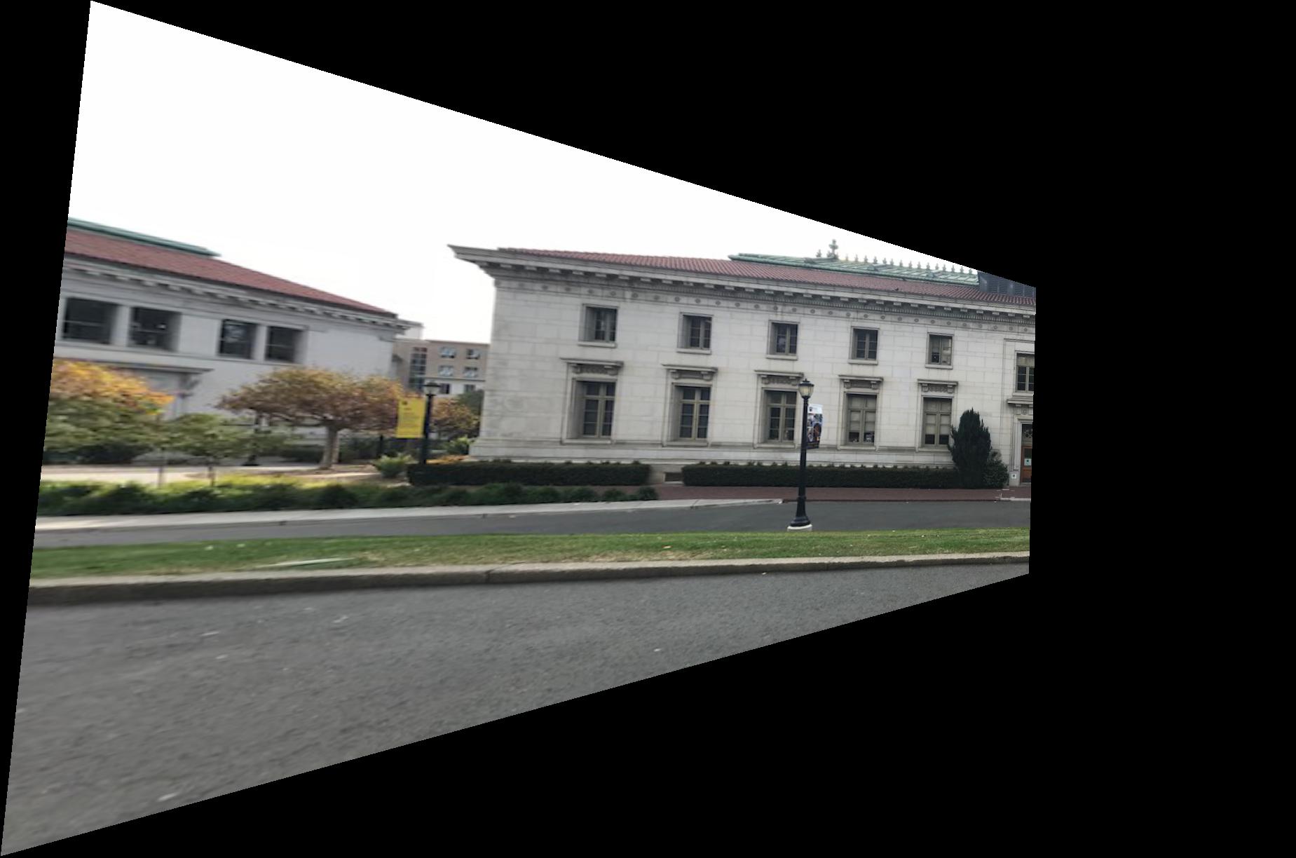
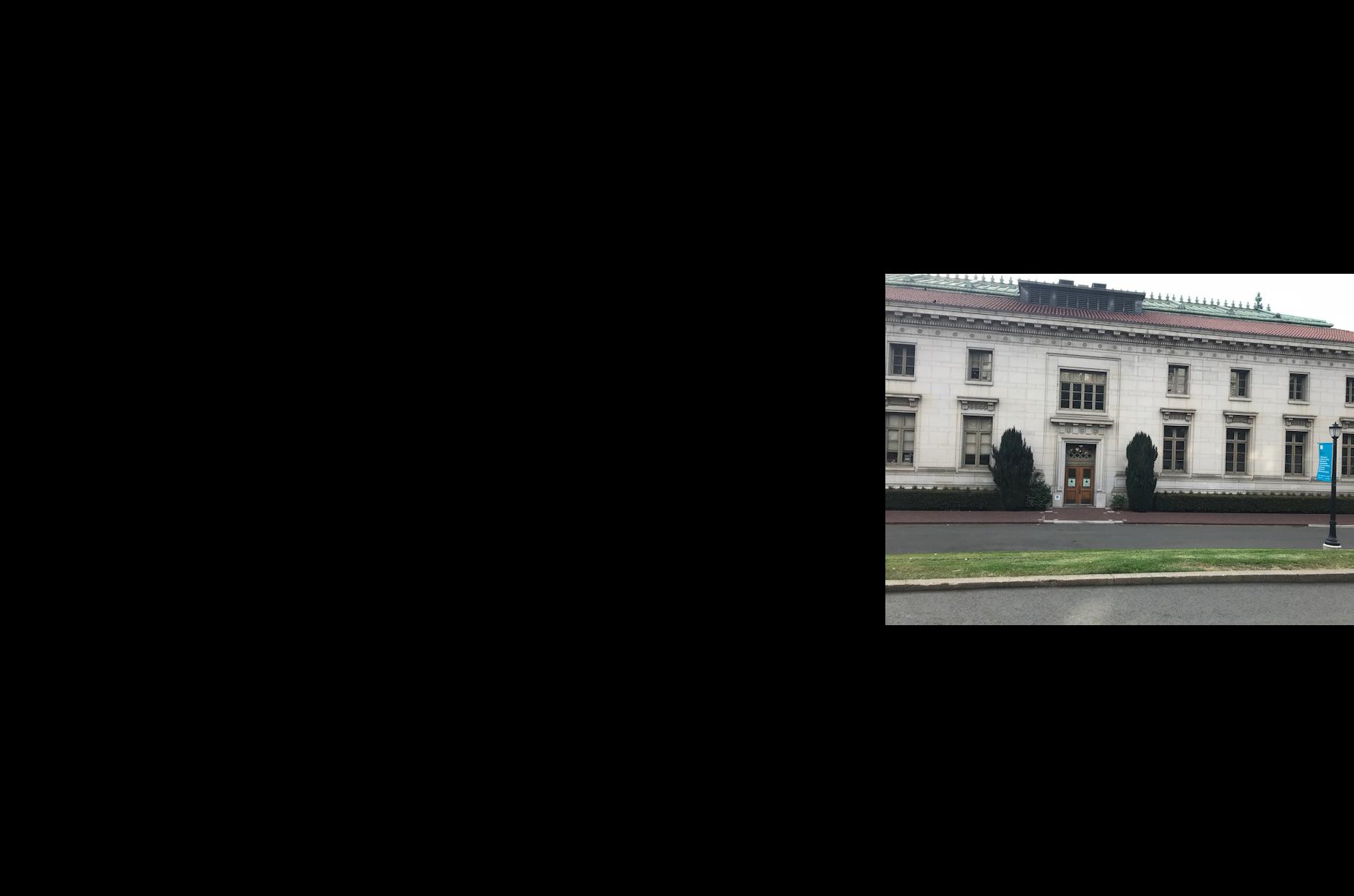
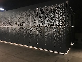
The process of creating an image mosaic is pretty similiar to the process of rectifying an image. However, instead of defining finding a homography between an image and a square, we find a homoraphy between two images. We then use this homography to warp the first image into the space of the second. After some tedious padding, shifting, and blending, my mosaics turn out as follows:
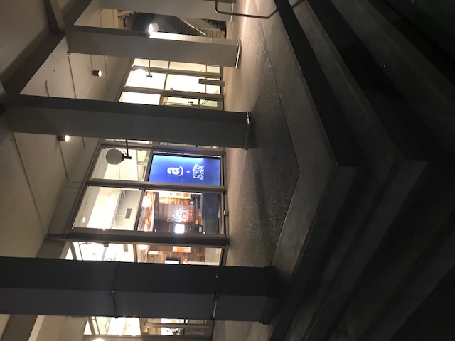
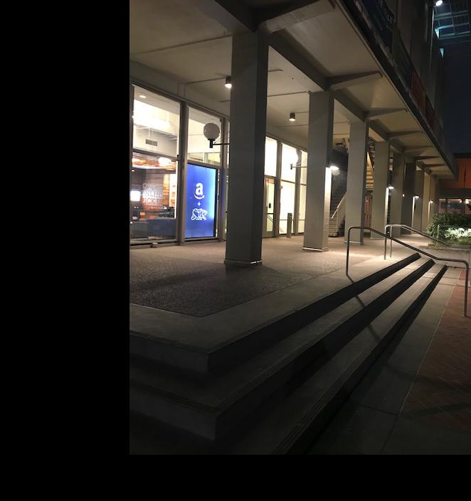
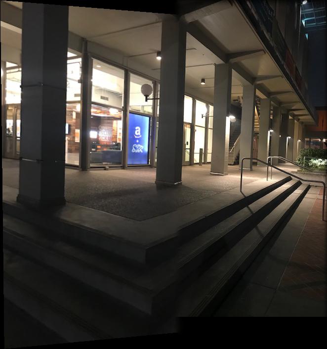
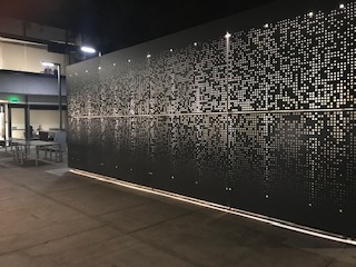
While there are still some visual artificats after blending (near the stairs), the darkness covers hides them up really well.
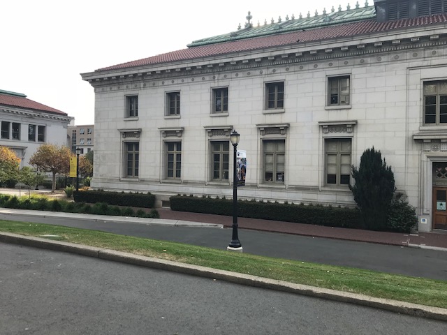
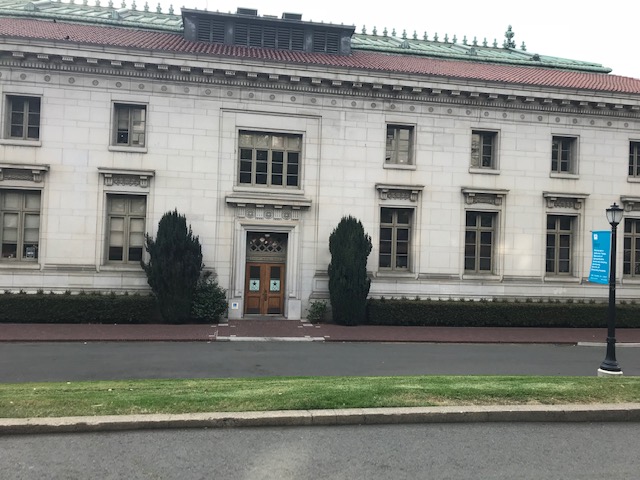
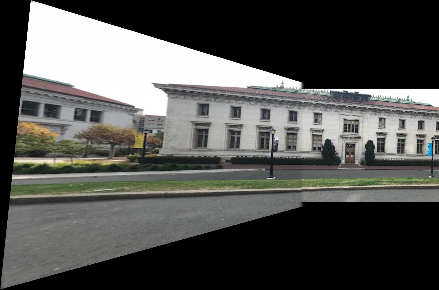
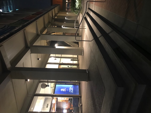
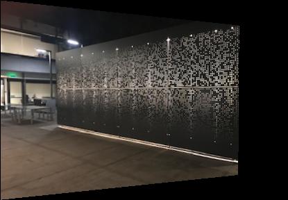
For this mosaic, the seam is visable due to the difference in lighting between both images. However, this color difference could be allievated by using Possion Blending instead of Laplacian Blending. Besides this, there is less visual artifacts than the previous mosaic.
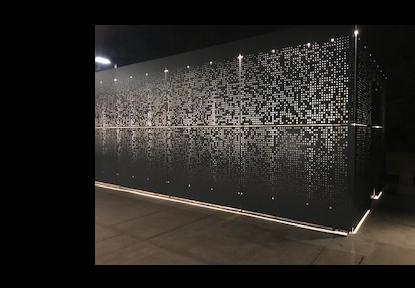
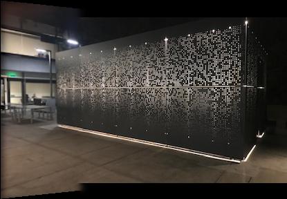
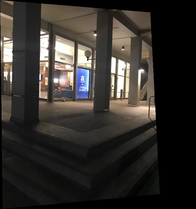
For this final mosaic, there really isn't much to say: the results turned out fine.
For the second part of this project, instead of selecting a set of correspondences and manaually computing a homography, we automate things using feature matching.
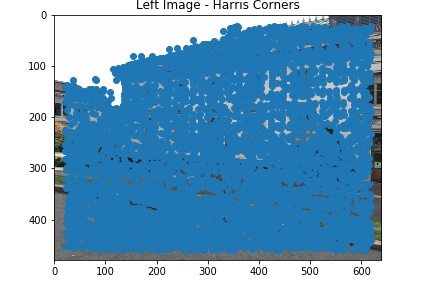
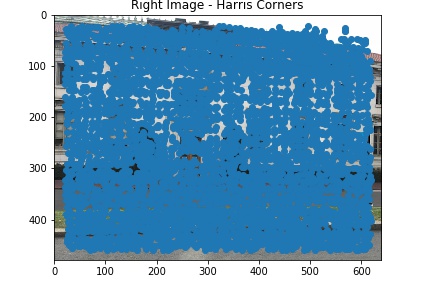
First, we use the Harris Corners algorithm to detect potential features. Harris Corners finds points with large corner response function R (R > threshold).
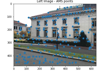
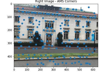
We have a set of interest points, however, we have too many. According to the MOPS paper, the cost of feature matching is superlinear in terms of the number of features. To reduce the number of points, while keeping them evenly distributed, we use ANMS. We define the maximuim supression radius ri for each point as follows:

The x points with the largest supression radius are retained. Using ANMS, I reduced the number of interest points to 200.
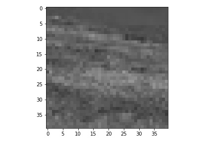
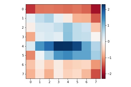
To extract a feature description for each point, we follow the procedure from the MOPs paper. For each point, we extract a 40x40 patch of pixels around the point from the image, and then subsample it into an 8x8 patch (accomplished with skimage's resize). Then we normalize the patch by subtracting its mean and dividing by its SD. Normalizing each patch makes it invariant to affine changes in intensity. Below I show an example of a feature patch along with its subsampled normalized version:
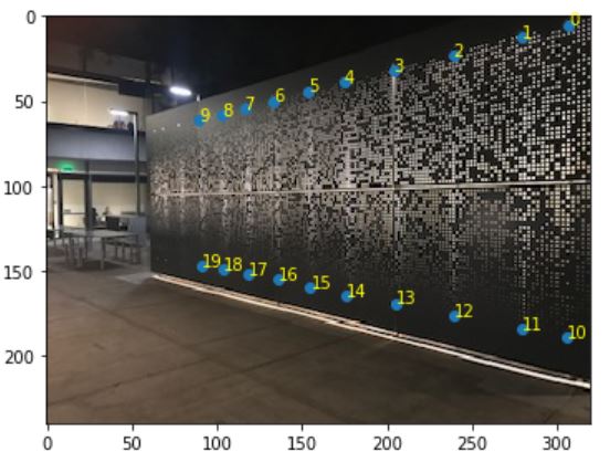
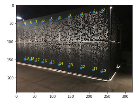
With our refined features and 8x8 image descriptiors, can begin image matching. We use Lowe’s technique introduced in MOPs paper: We consider a pair of features f1 and f2 from 2 different images a match if the the ratio e1 / e2 is larger than some threshold. Here, e1 is the error from f1 to its nearest neighbor patch in the second image (f2), and e2 is the error from f1 to its second nearest neighbor patch in the second image. Using Ajay's Visualizer code from Piazza, we can visualize our set of matches:
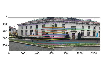
As evident from the previous part, multiple outlier are still present in our matches. To reduced the number of outliers, I use RANSAC to estimate the homography. This works by selecting