Part A: Image Warping and Mosaicing
Overview
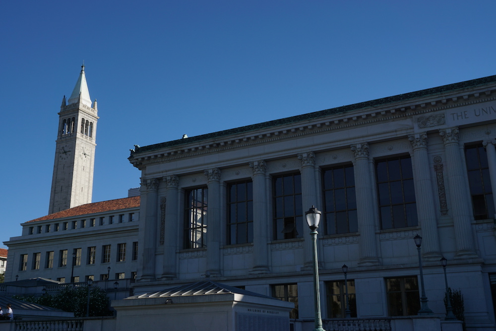
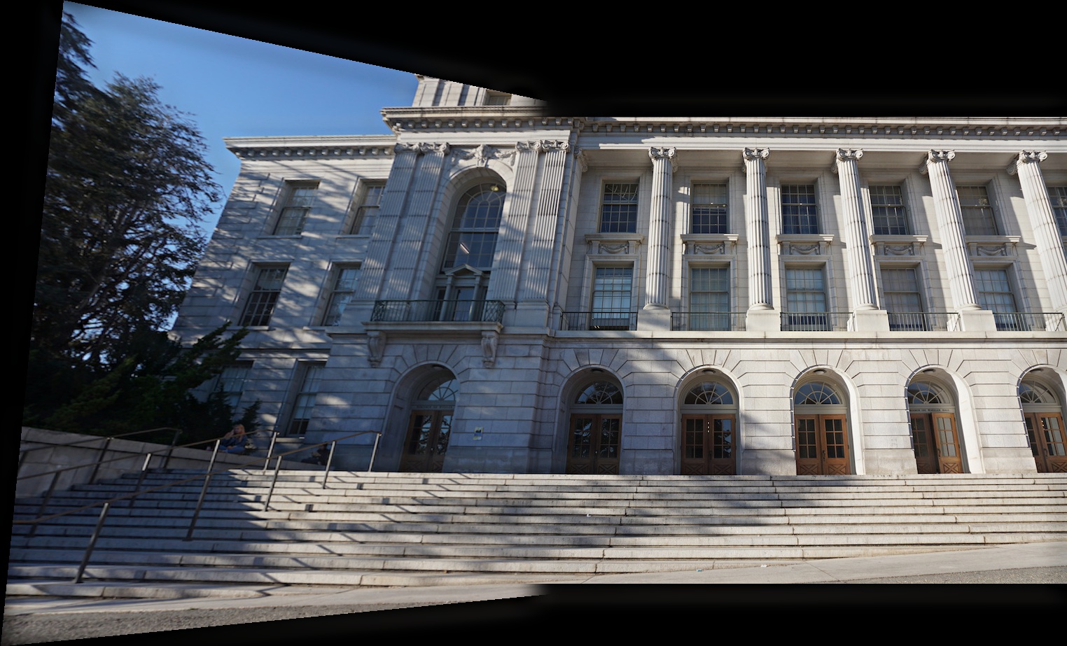
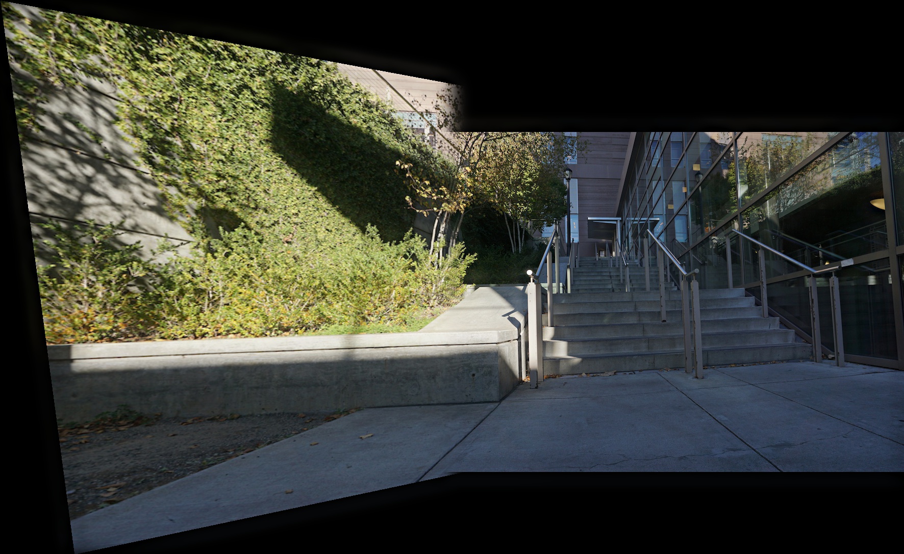
In this part of the project, we aim to utilize image warping to implement image mosaicing. By calculating the homographies, we are able to combine images taken with overlapping fields of views views from the same point, but with the camera rotated to point at different angles, and stitch them into a single image utilizing projective morphing.Shoot the Pictures
Recover Homographies
The homography transform follows the following equation where H is a 3x3 matrix, where i = 1 and thus has 8 degrees of freedom. x and y are the original point, whereas x' and y' are the point following the transformation. Thus, we recover the homography by attempting to find H in the following equation.
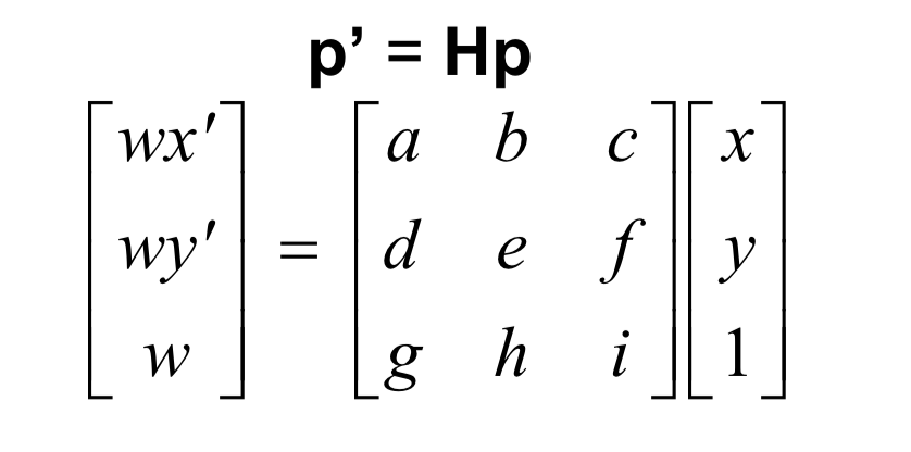
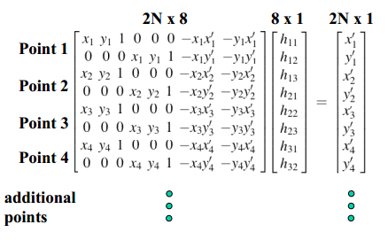
Image Rectification
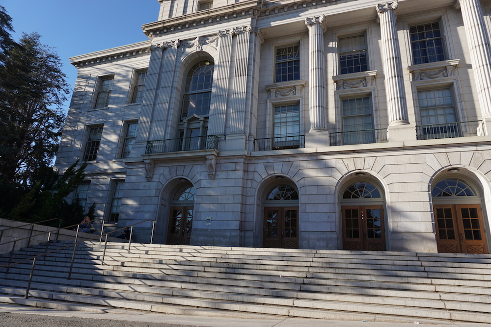
Using the recovered homographies, we can warp the images to rectify the images. Warping the image is achieved by mapping the four corners of the original image through the homography transform to obtain the four corners of the result image and calculate the size. Then, for each pixel in the resulting image, we can calculate the pixel's value by using the inverse of the homography matrix to identify where we should sample the original image. Using interp2d, we are able to avoid aliasing the image and retrieve the pixel value for the position. To rectify planar images, I selected points with a known shape (i.e. windows and doors are rectangular) to generate the points the image should be warped to when generating the homography matrix H.
Doe
Wheeler
Doe Rectified
Wheeler Rectified
Blend into Mosaics
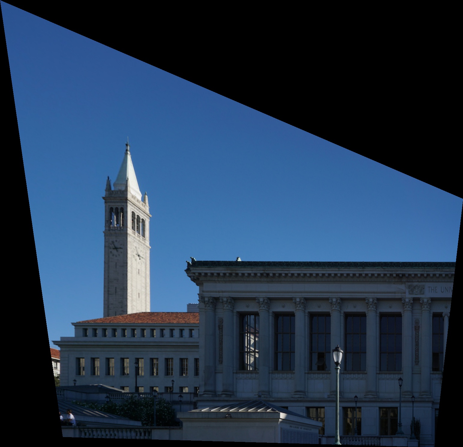
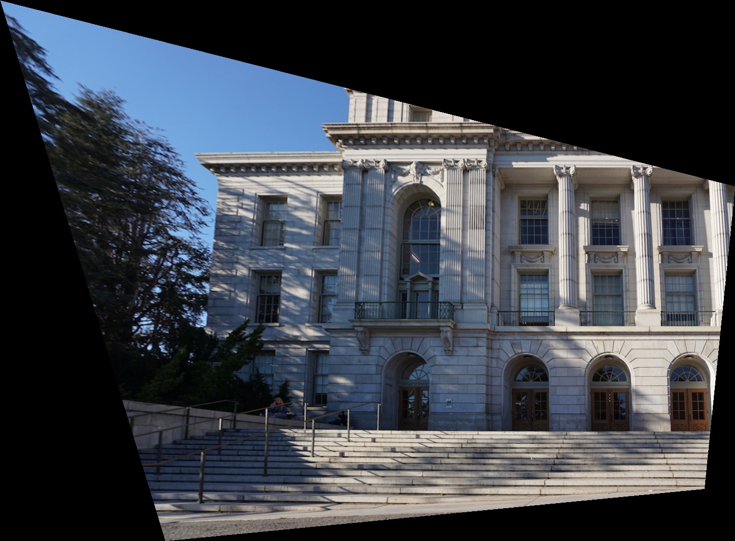
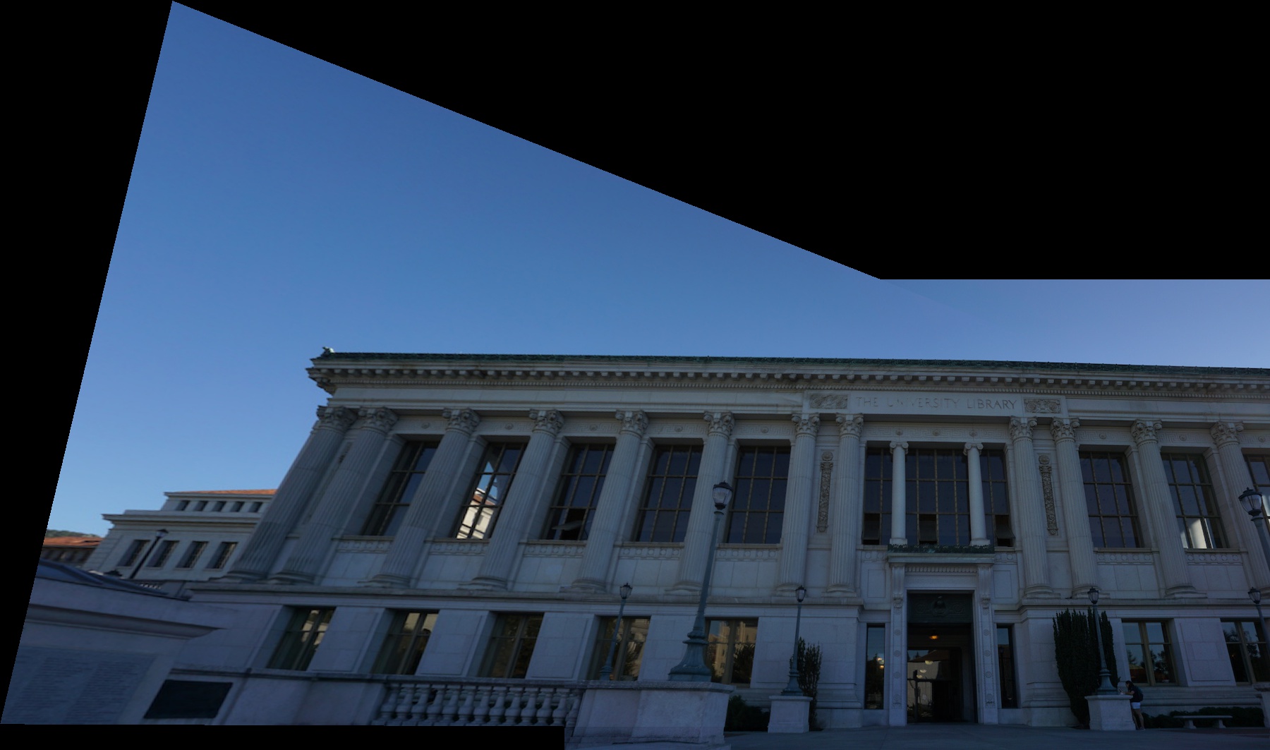
To blend two images together into a Mosaic, I computed a homography matrix to transform the points selected from the left image (im1) to the corresponding point coordinates selected from the right image (im2). We can then use the inverse homography transform similar to our image rectification to compute a warped version of image 1. To combine the two images together, using element-wise maximum over the pixels from each image for overlapping regions produced a fairly seamless blend without introducing unnecessary blurring that can result from alpha-blending.
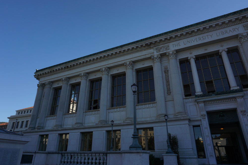
Doe 1
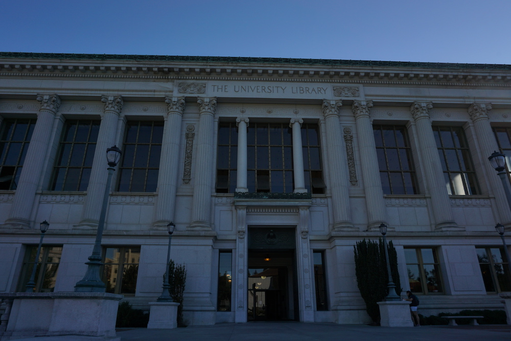
Doe 2
Doe Merged

Wheeler 1
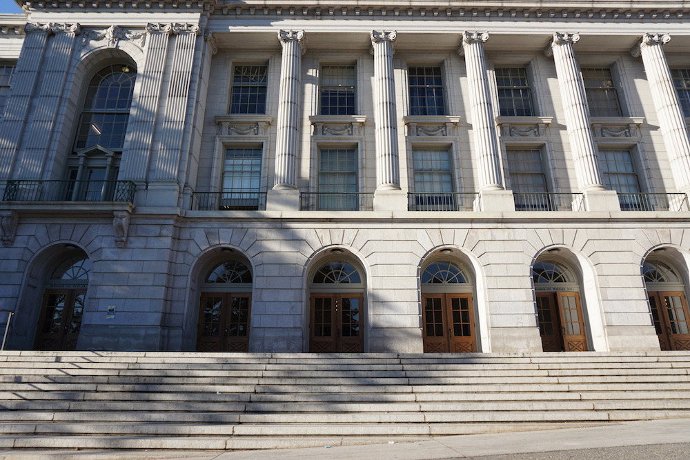
Wheeler 2
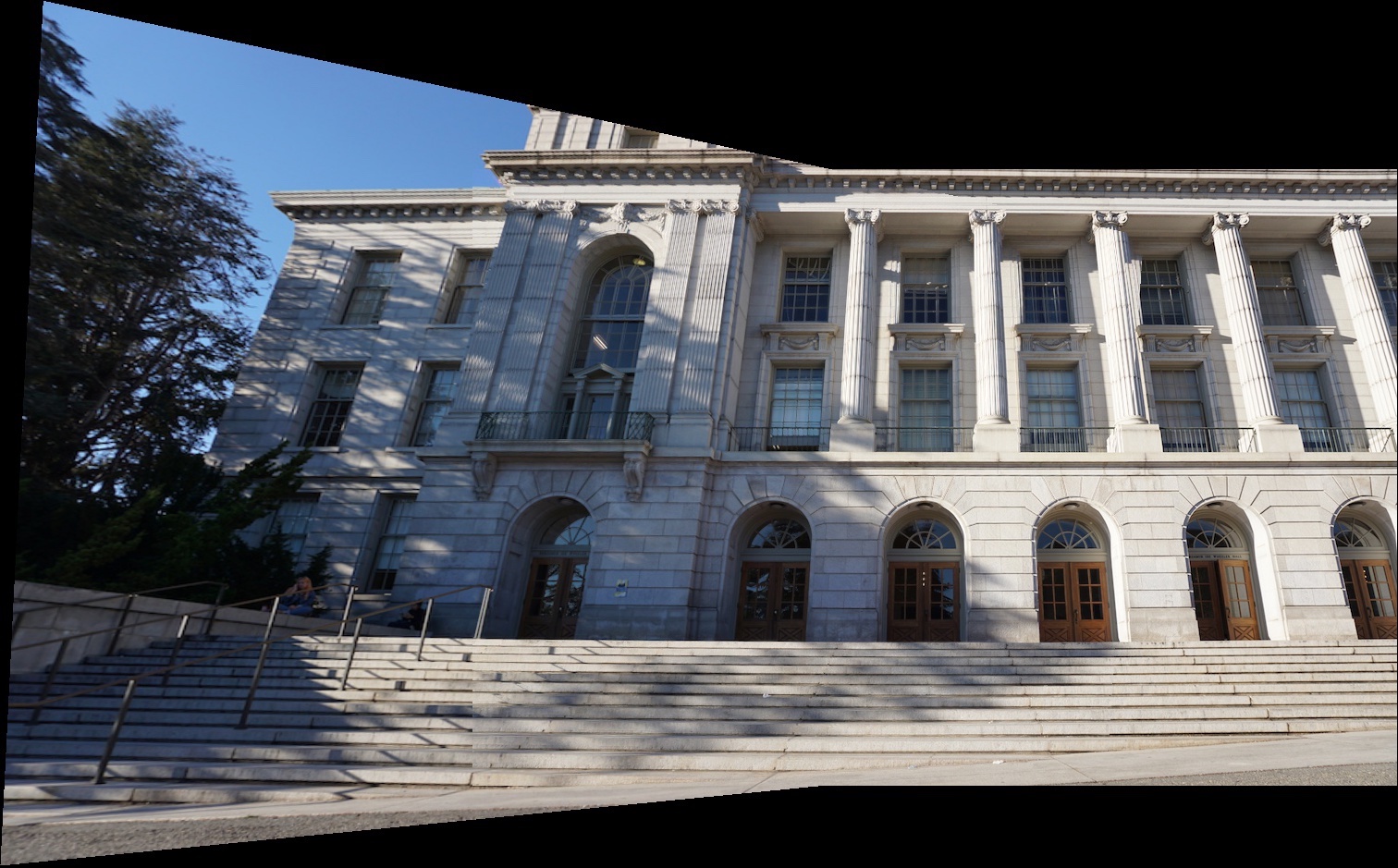
Wheeler Merged
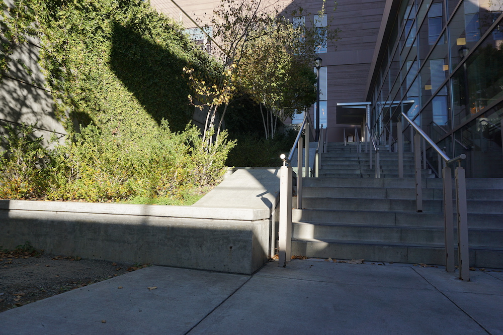
Steps 1
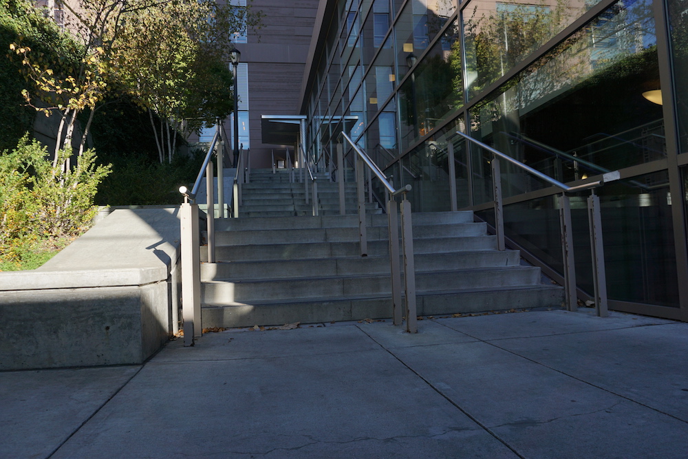
Steps 2
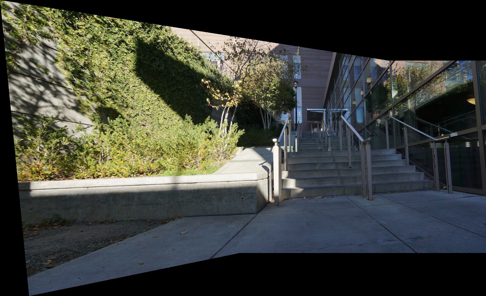
Steps Merged
Summary
From this project, I learned the importance of linear algebra and how relatively simple systems of linear equations can yield powerful transformations that can alter images and perception.
Part B: Feature Matching For Autostitching
Overview
In this part of the project, we aimed to automatically detect good, matching feature points in our two images to utilize for homography calculation to improve image warping and mosaic stitching from part A to improve precision and reduce human error.
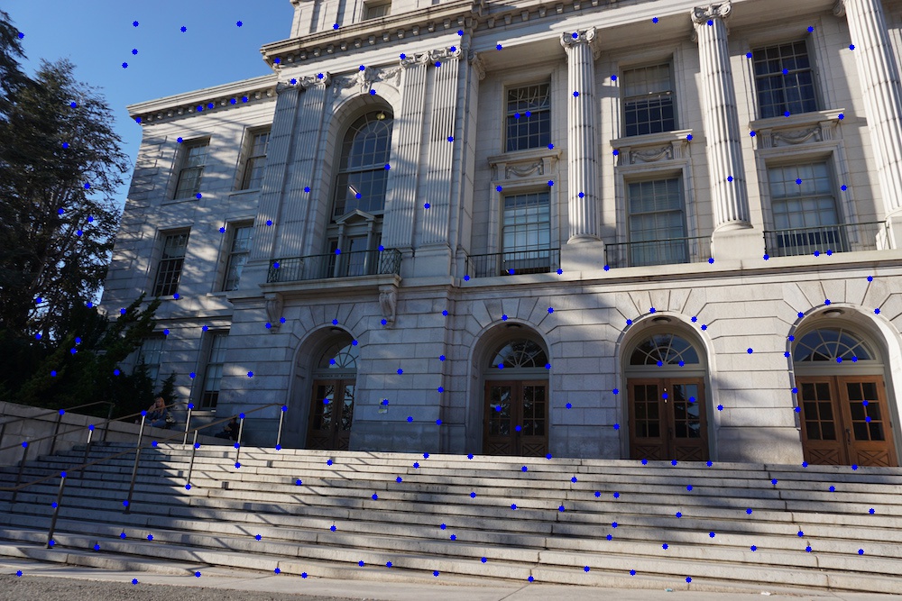
Detecting Corner Features
We utilize harris corner detection on the greyscale image to find corners for the image where the image region as different edge directions. By limiting the min_distance to 10, we get the following points (overlayed on the image below).
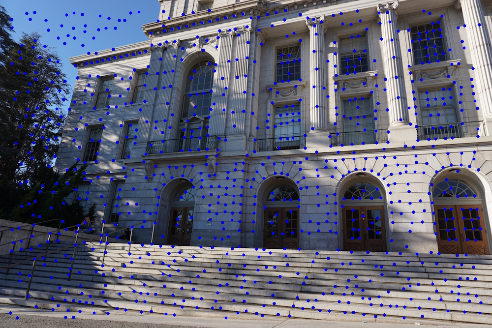
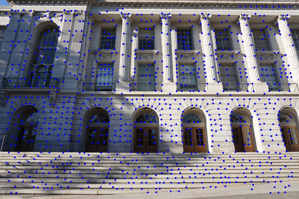
We can then utilize Adaptive Non-Maximal Suppresion to reduce the number of interest points to 200 points. This was done by iteratively decreasing the radius r, and for each radius r, finding the points that have a larger harris value than every other point within the radius by a scaling factor, crobust, of 0.9, until we have found the appropriate number of points. Following this process, we were able to reduce our interest points to the following points.

Extracting A Feature Descriptor For Each Feature Point
To represent each feature point, we generate feature descriptors by sampling 8x8 patches from a larger 40x40 window by using every 5th pixel followed by applying a bias/gain-normalization for a 0-mean and 1-std.
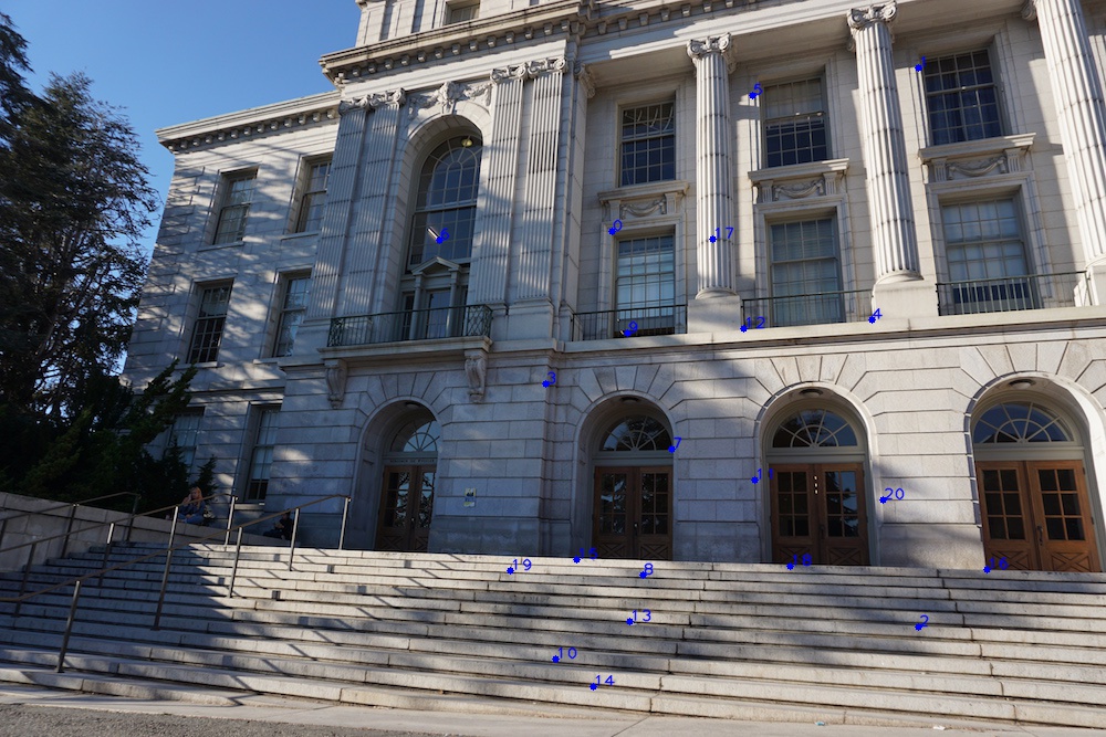
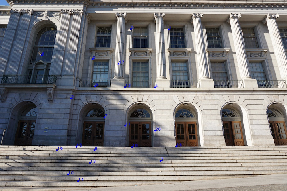
We then use these descriptors flattened into a 1 x 64 vector to indentify feature matches between the two images by finding points whose descriptor has the best match, using SSD. If the best match is much better than the second-closest neighbor, we consider these two to be a match. Below are the matching points shown for two images of Wheeler.


Use a Robust Method (RANSAC) to Compute a Homography
After limiting our feature points and finding several matches, we can use RANSAC to find a subset of matches to use for our homography calculations. We do this by randomly selecting four points, computing a homography matrix, and seeing how many points work well with that homography (i.e. are inliers). We then maxmimum inlier set as the points for our final homography calculation H. Note that some of the points from the previous matched points have been discarded below.
Proceed as in Project 3 to Produce a Mosaic
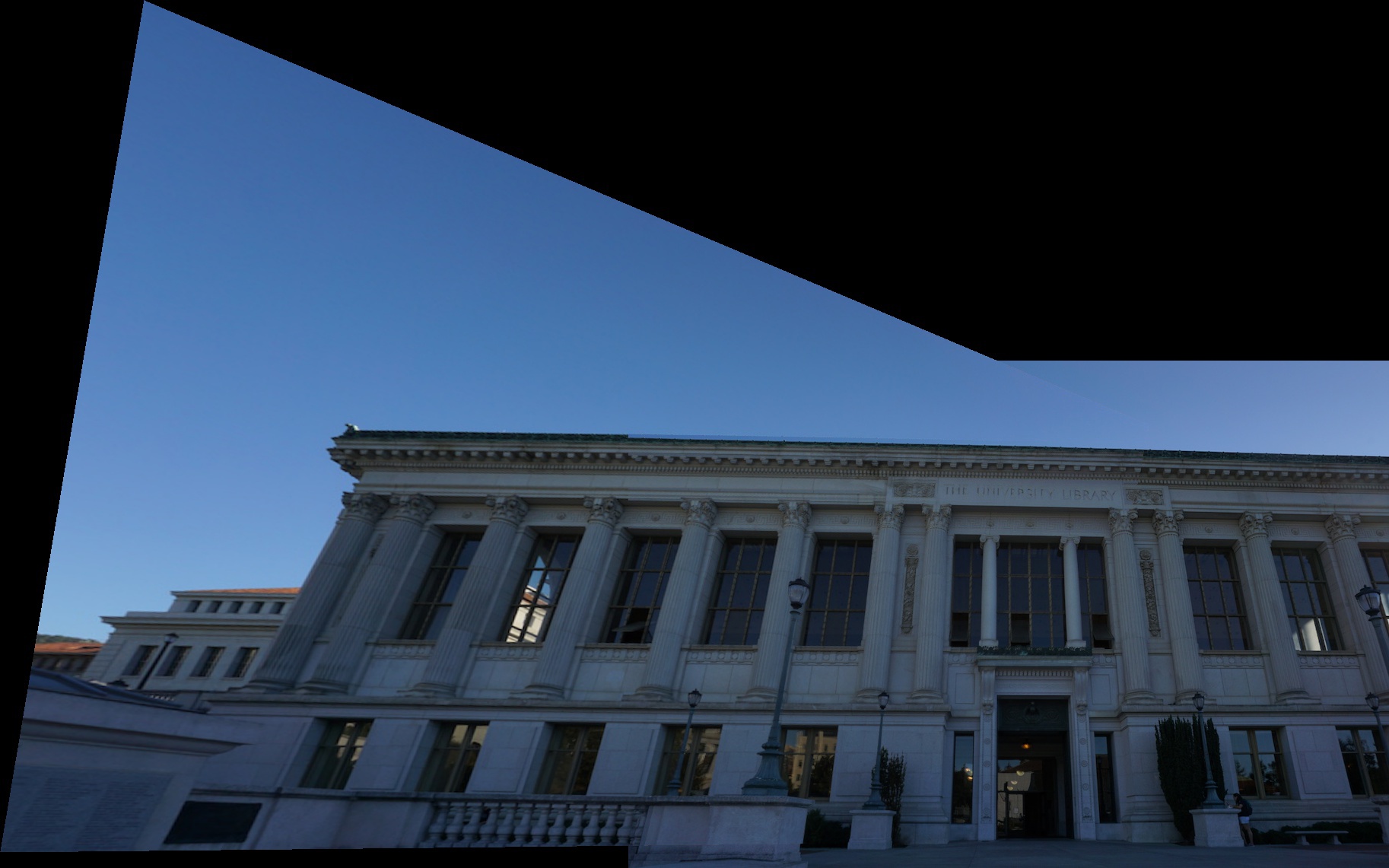
Using our final homography matrix H as produced from RANSAC, we can apply H in the same manner as part A to generate our automatically stitched mosaics. Below, we show the automatically stitched mosaics compared to the manually stitched mosaics from part A. To aid with blending, I also added multiresolution blending along with the max-merging from part A to reduce artifacts from merging (used for Wheeler and Steps)
Doe 1
Doe 2
Doe Manual Merged
Doe Auto Merged
Wheeler 1
Wheeler 2
Wheeler Manual Merged
Wheeler Auto Merged
Steps 1
Steps 2
Steps Manual Merged
Steps Auto Merged
Summary
Doe 1
Doe 2
Doe Manual Merged
Doe Auto Merged
Wheeler 1
Wheeler 2
Wheeler Manual Merged
Wheeler Auto Merged
Steps 1
Steps 2
Steps Manual Merged
Steps Auto Merged
From this project, I learned that point-detection and selection/matching schemes can use SSD to find points of interests without human input and can generate merged mosaics just as good as humans. This method reduces human-error and makes generating mosaics much faster without compromising accuracy.