I took a series of photographs of different subjects, where I kept my camera in the same location but
rotated it after each picture to capture a wider field of view.
I created a small wrapper around ginput to allow the user to input correspondences between
images, and proceded to use the tool to find correspondences between each successive pair of photographs
in each set.
I also took a few individual images that had rectangular objects or planes in them, to use to
test my homography finding code and image warping code.
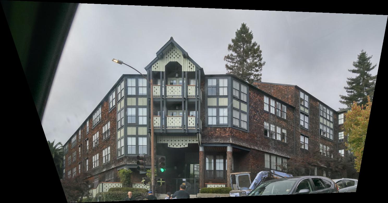
I used a similar ginput based tool to define four corners of a rectangle within each image,
and then compute the homography to fix the angles of the quadrilateral to 90 degrees each:
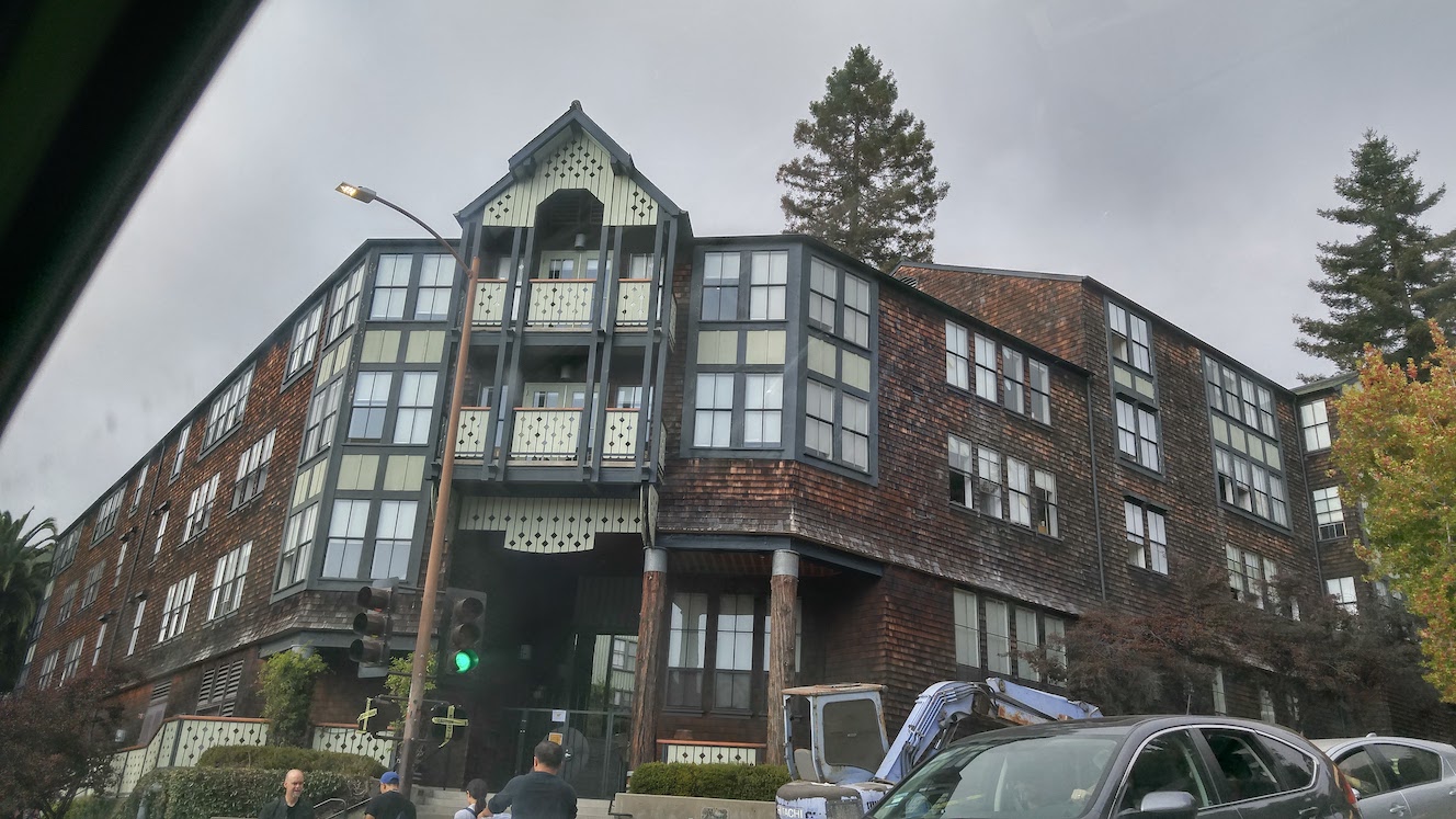
Foothill
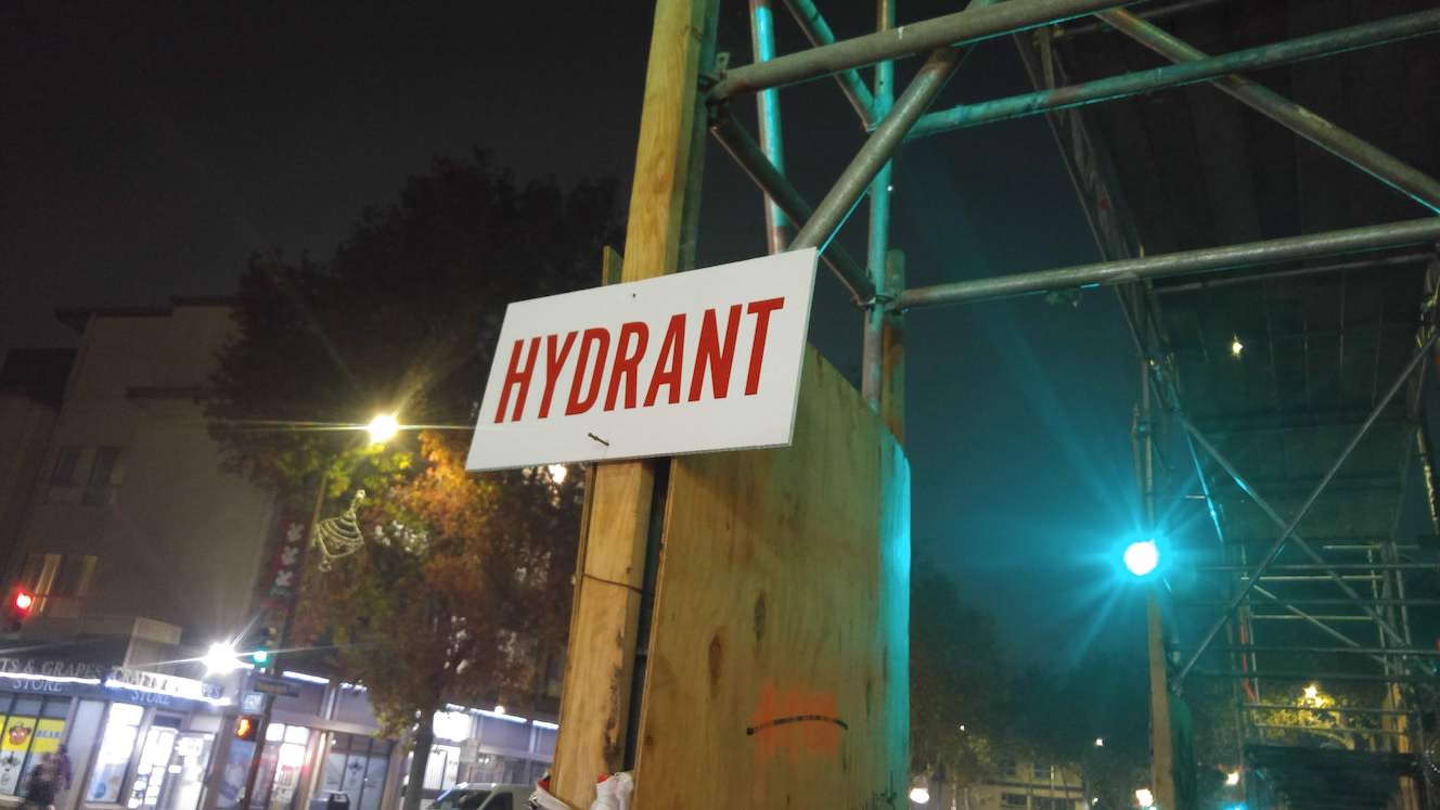
Sign on Telegraph Ave
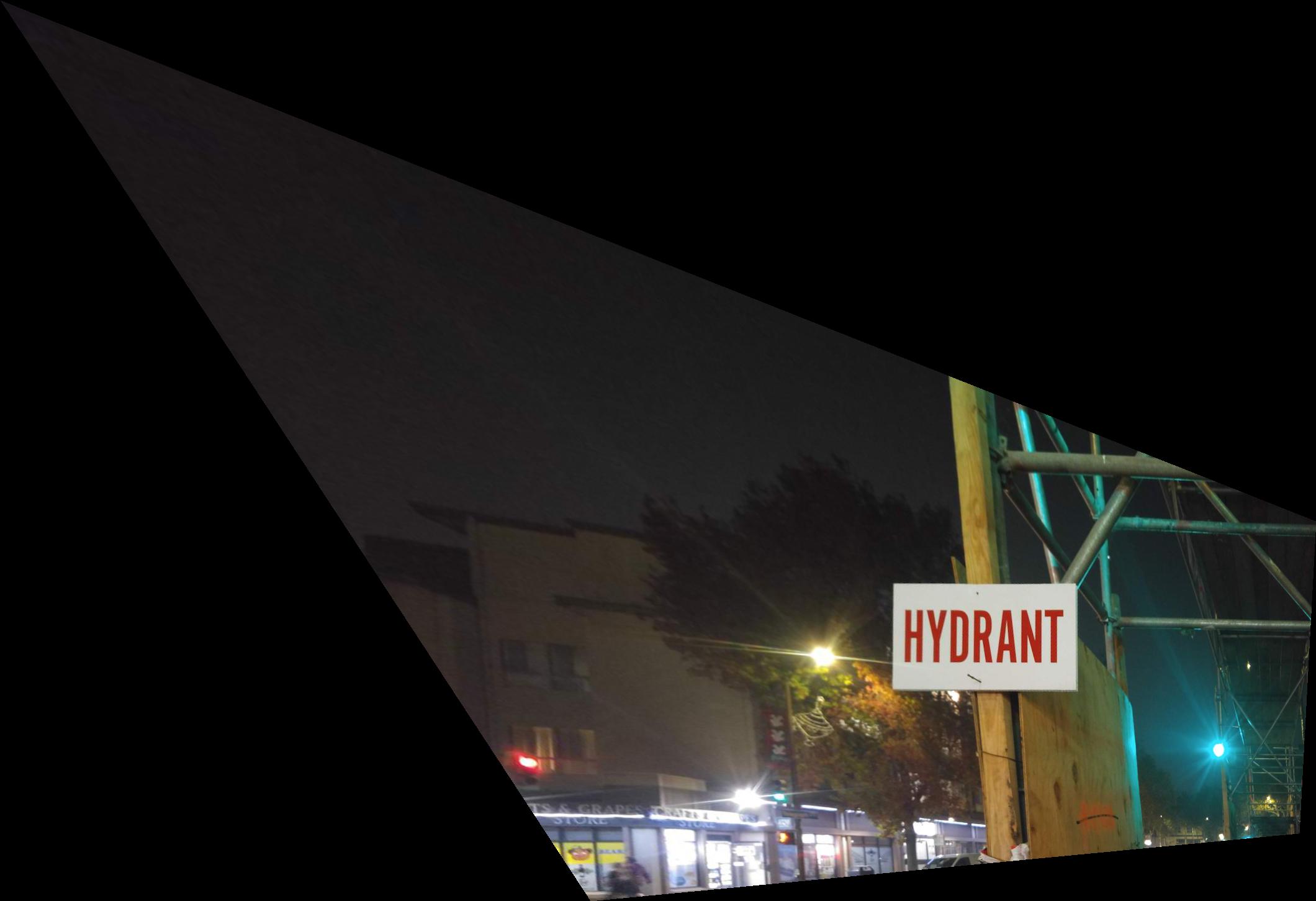
I rectified the front face of Foothill on the left, and the "Hydrant" sign on the right.
I recommend clicking on each image to view it in full size:
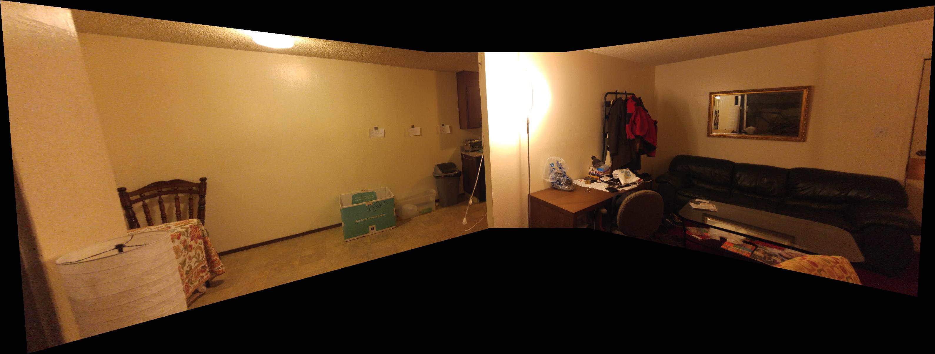
Using the correspondences defined previously, and the function to compute the homography matrix and transform an image, I created
three panoramas of three photographs each, where the left and right image were both warped to the projection of the center image.
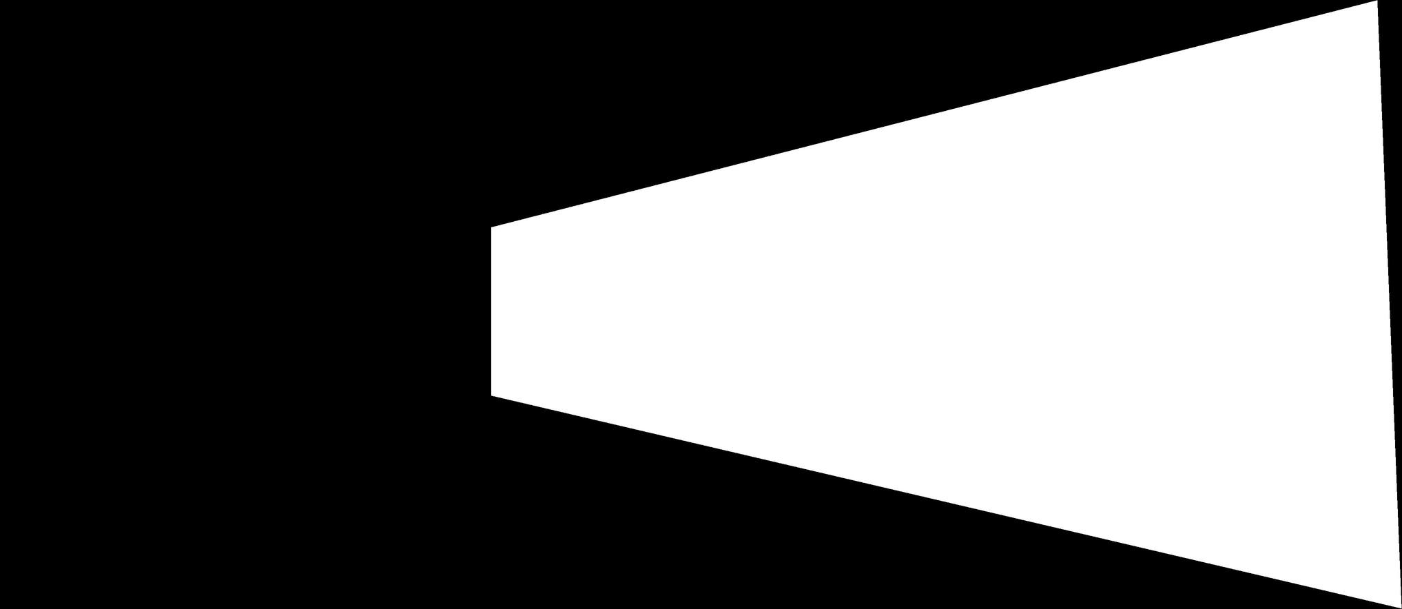
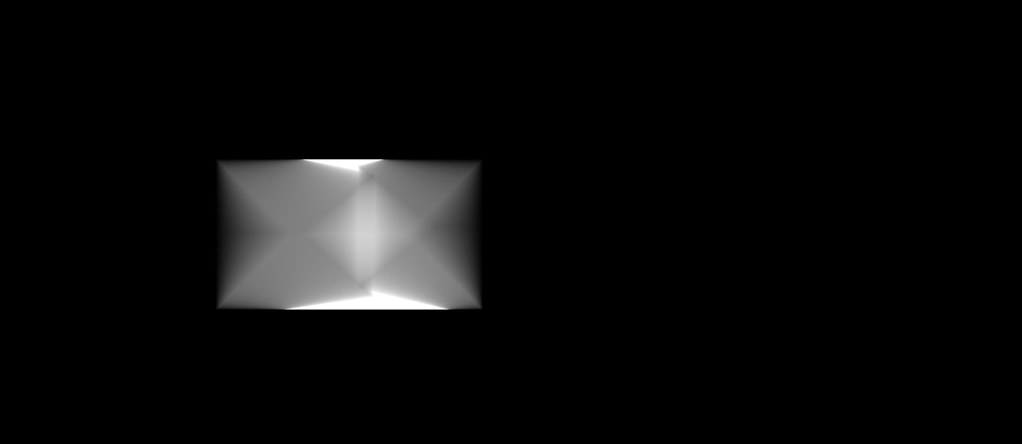
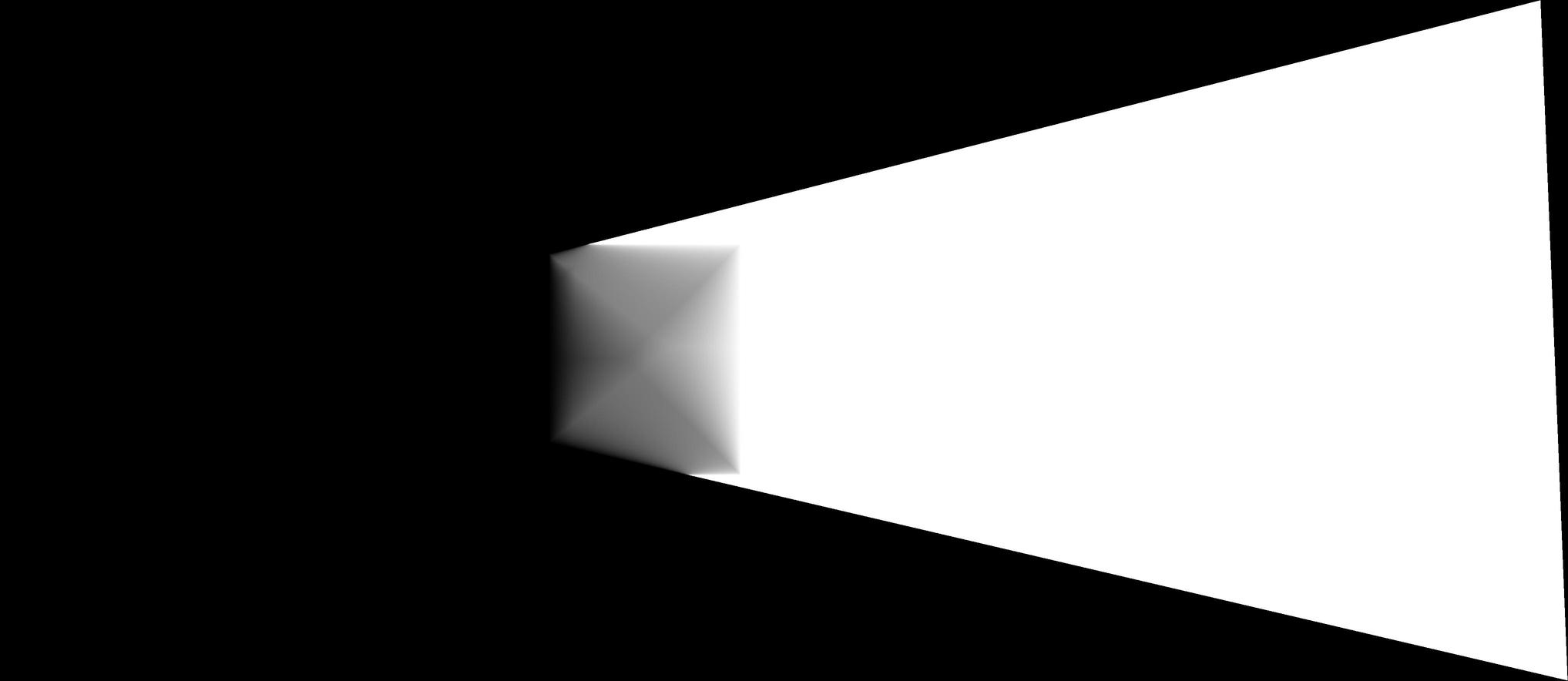
To actually blend the three separate transformed images, I first took the binary masks of each of the transformed images:
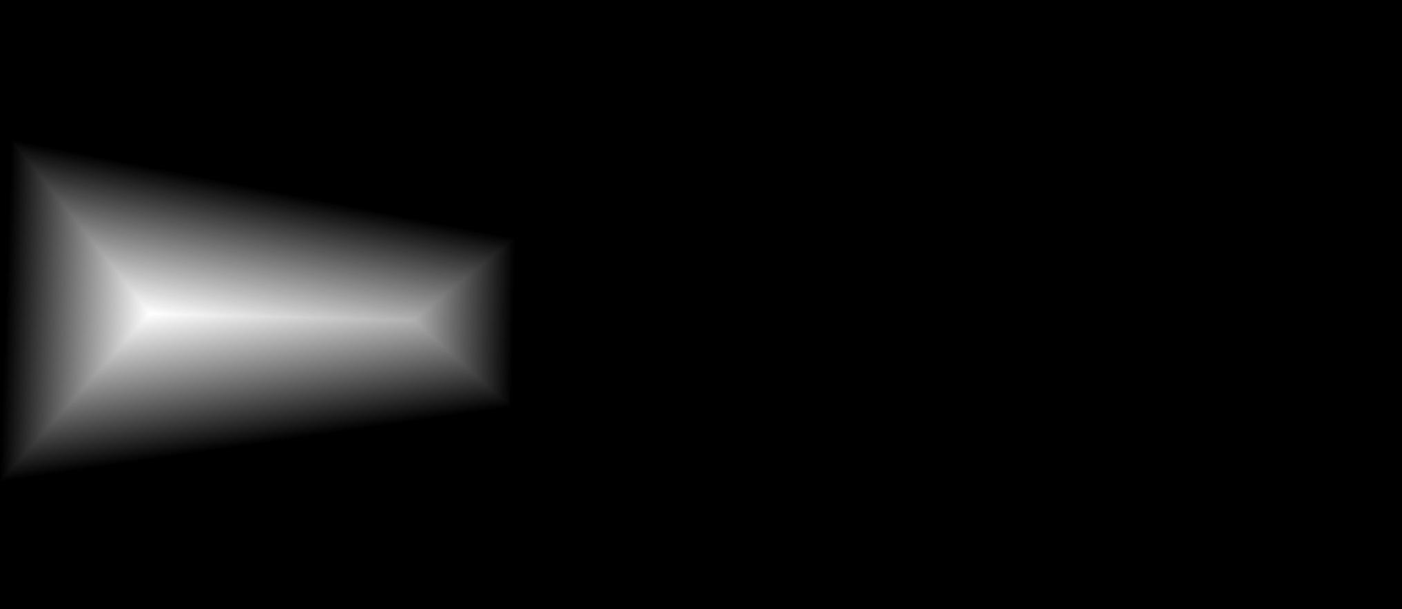
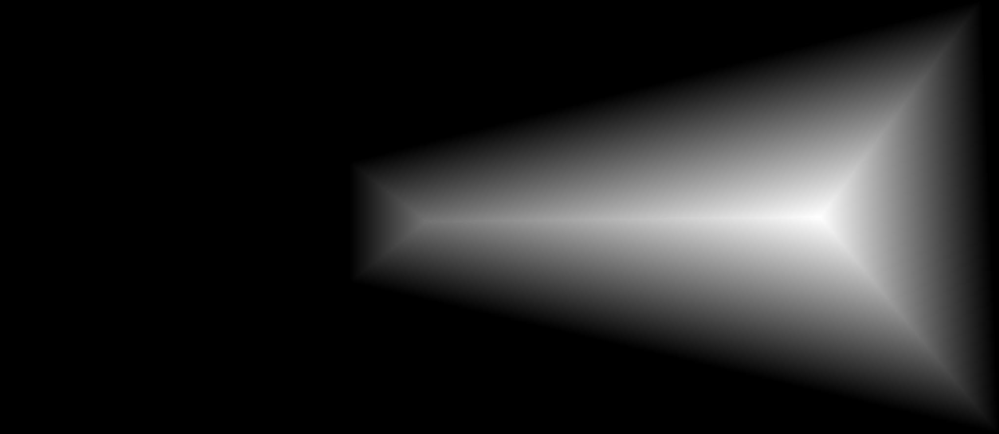
Then I computed for each white pixel the distance from the nearest black pixel, to get a smooth fade in each of the masks:
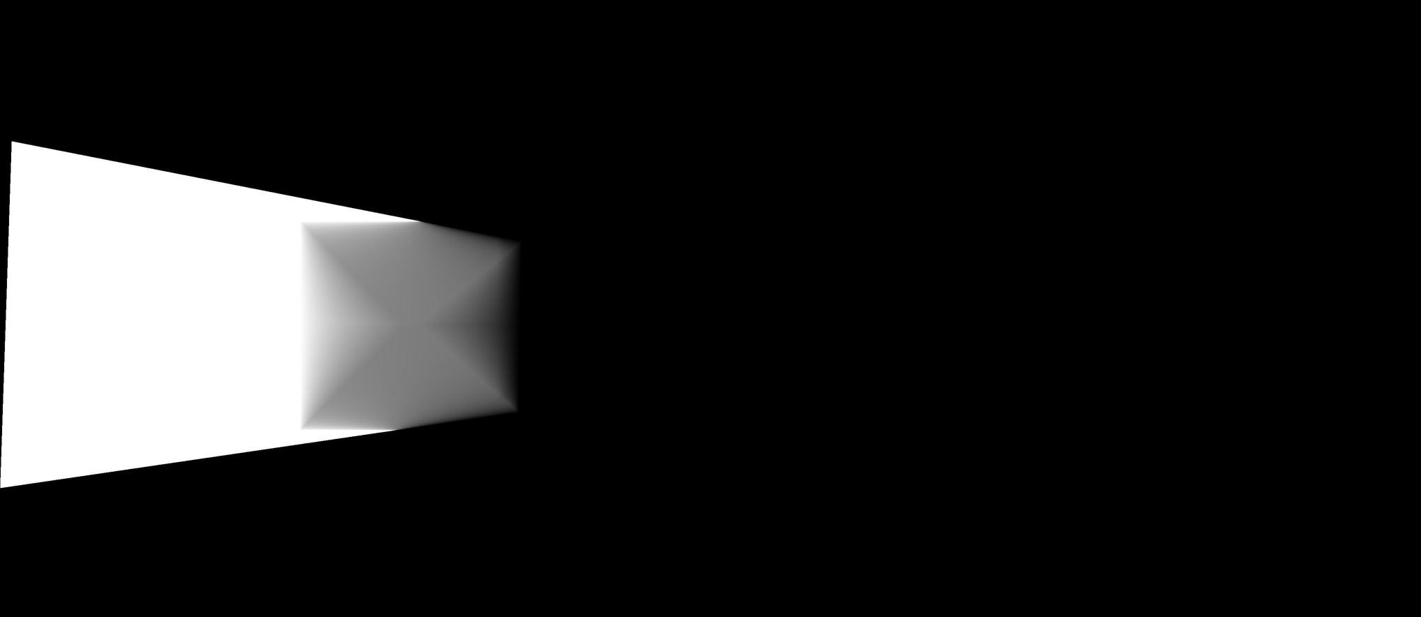
And then I summed each of the masks and normalized them against the sum, to get a mask which could be multiplied
component-wise each each of the respective transformed source images before summing them together.
There are some weird wedge artifacts in the distance fields due to the sharp shape of the masks, but
it still ends up blending well.
Before this project, I didn't realize just how distorted the edge of the field of view gets with perspective.
It makes sense that fisheye lenses have such severe distortion due to needing to squeeze a large amount of image into
a small area (the edges of the frame).
I was also trying to stitch together more than 3 images -- but the transformation that would be applied
to another image in the sequence was just so severely stretched (probably due to reaching approximately
a 180 degree field of view) that it didn't work -- the final image would have ended up being millions of pixels across.
I also tried to stitch together some pictures I took a year or two ago at a train station, but the correspondences never
ended up actually lining up -- it seems that I must have moved too much while taking the pictures.
After implementing stitching that works with hand-defined correspondence points,
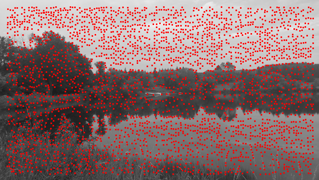
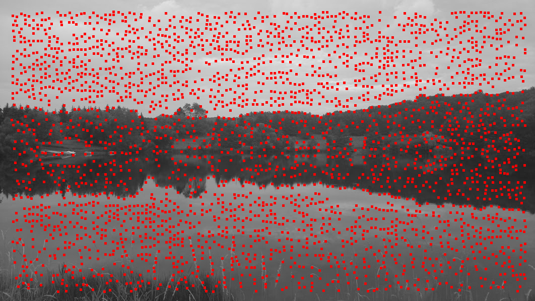
I implemented a simplified version of the Multi-Scale Oriented Patches (MOPS) algorithm
to automatically find and match features across images for computing a homography.
Next, I downsampled by images by 5x, and extracted an 8x8
region around each sample point (having the effect of taking a 40x40 pixel
region, low-pass filtered and downsampled to 8x8).
Then, I normalized each feature descriptor by subtracting by the mean
and dividing by the standard deviation.
Then, I found candidate matches between the features of the two images.
For each feature in the left image, I computed the nearest neighbor (1-NN)
and second nearest neighbor (2-NN) by the SSD metric. There is a match
between the feature and its 1-NN if the ratio of the distance to its 1-NN
to the distance to its 2-NN is smaller than 0.5.
After finding candidate matches, I ran RANSAC (10,000 iterations):
four matches would be chosen at random, a homography would be computed with them,
and then each of the other points from the first image would be transformed with this homography.
The set of points that were transformed to within 5 pixels of their corresponding
point in the second image are considered to be the inliers -- the largest such
set of inliers at the end of the iterations is taken to be the "true" homography.
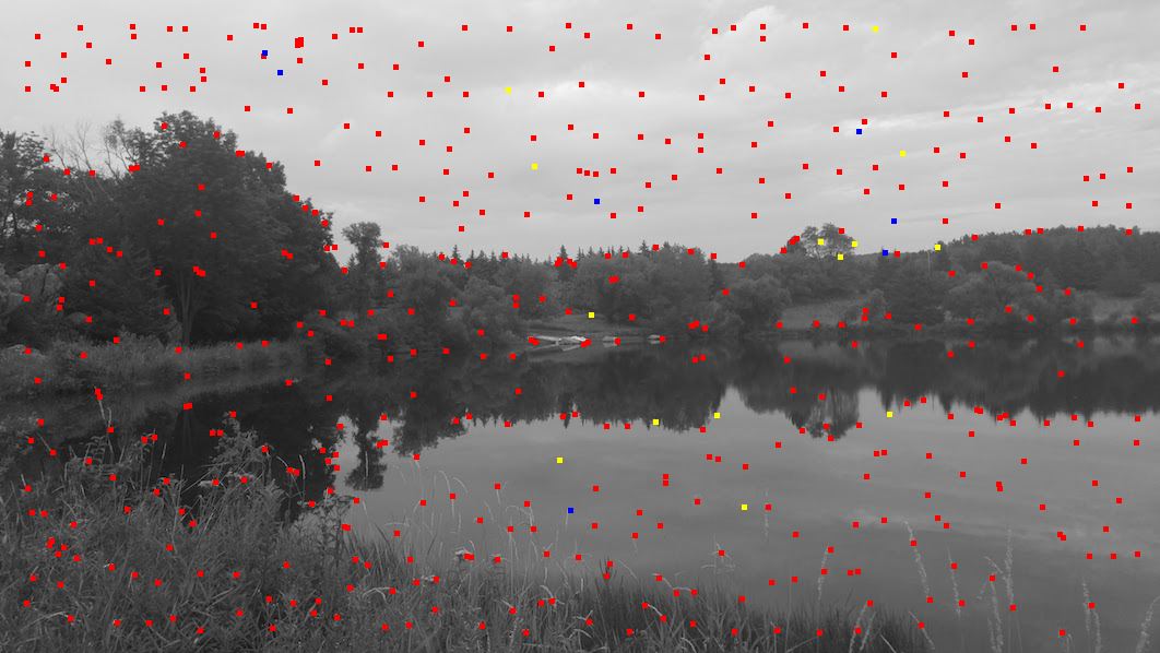
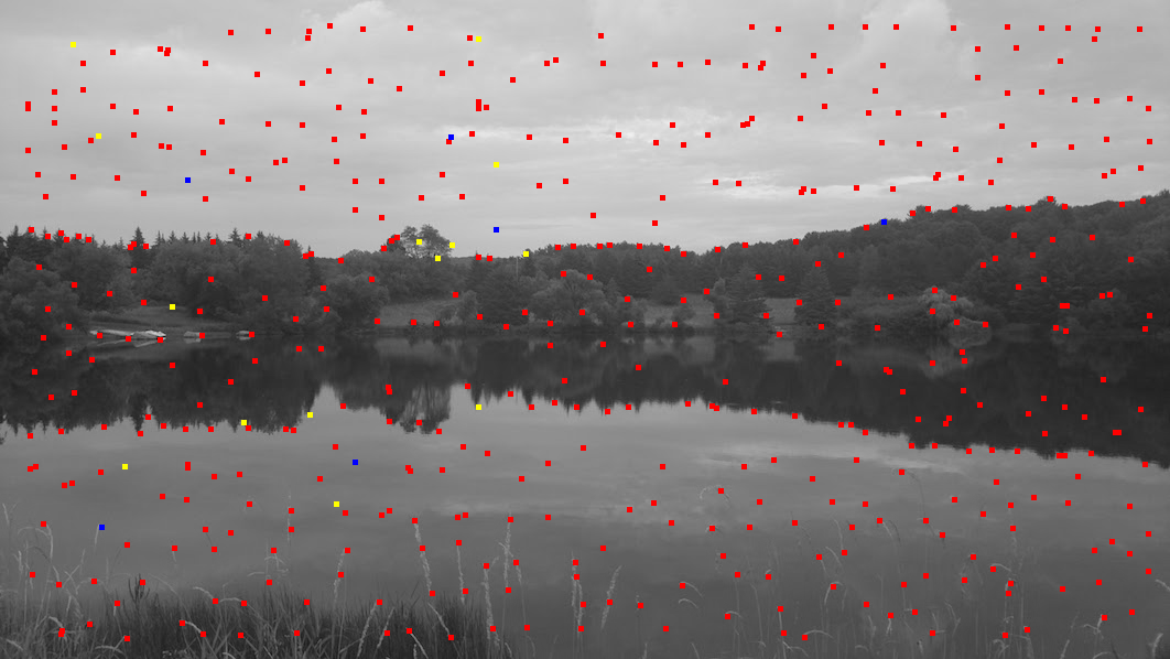
In the images above, red points are feature points that did not have any match in the other image,
blue points are ones with matches that were rejected by RANSAC, and yellow points were matches
that were used in the computation of the final homography.
With the homography computed with RANSAC, the images were transformed and blended
together, as described above.
For each of the following images, the manually defined stitch is first, followed by the
automatic version.
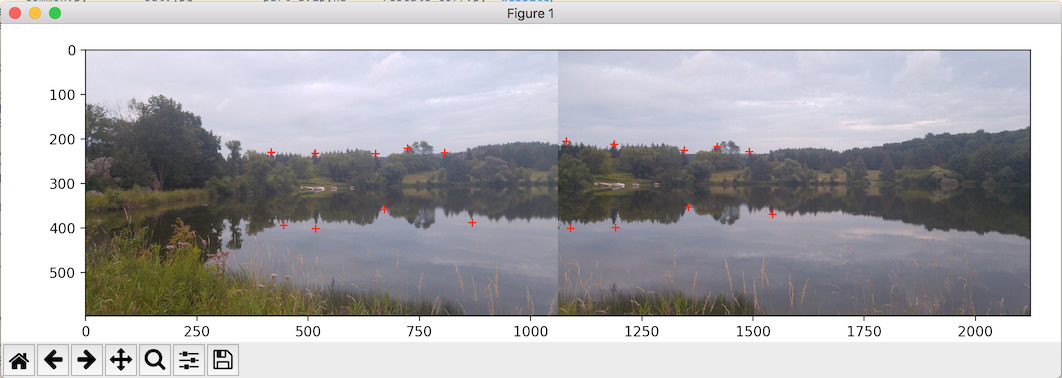
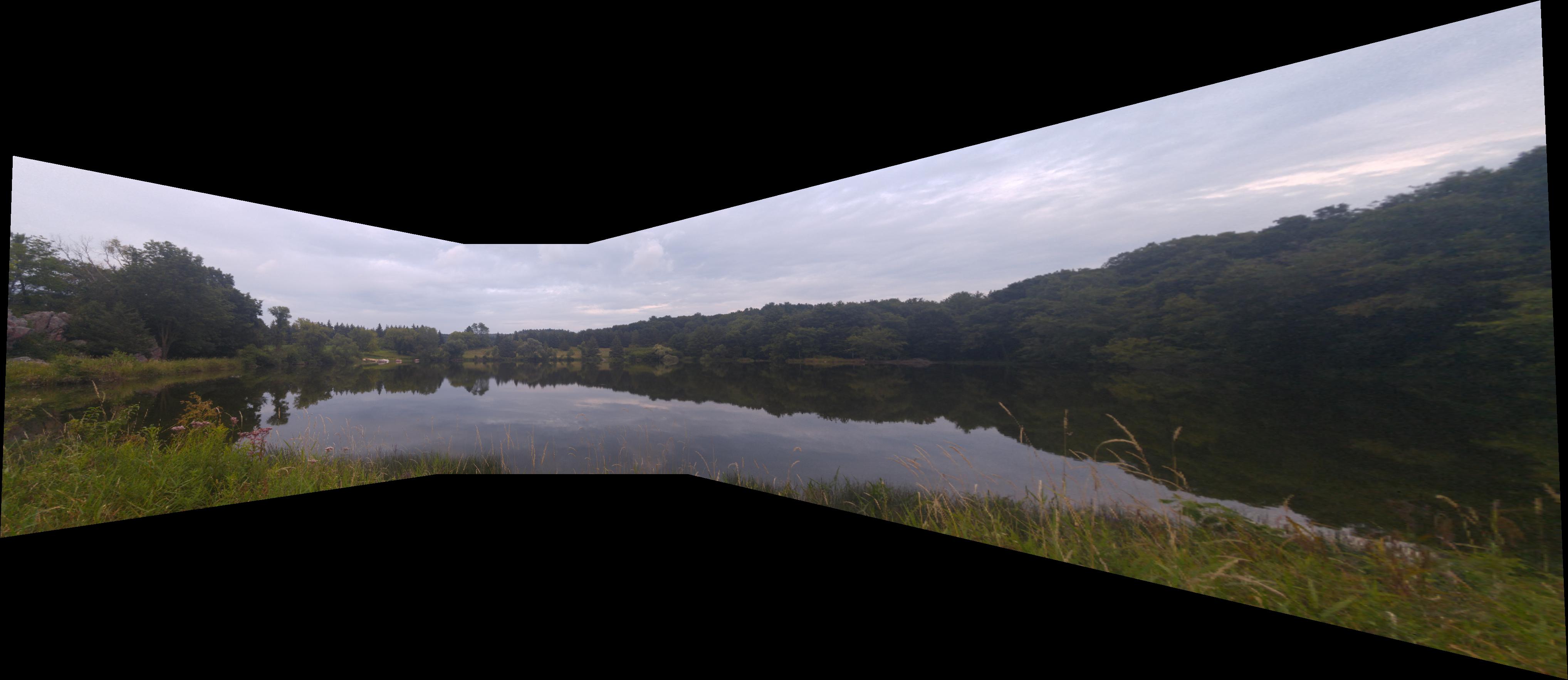
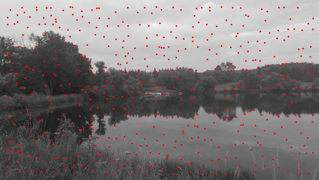
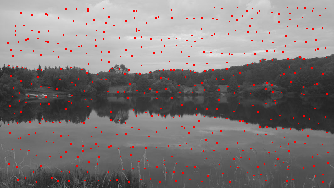
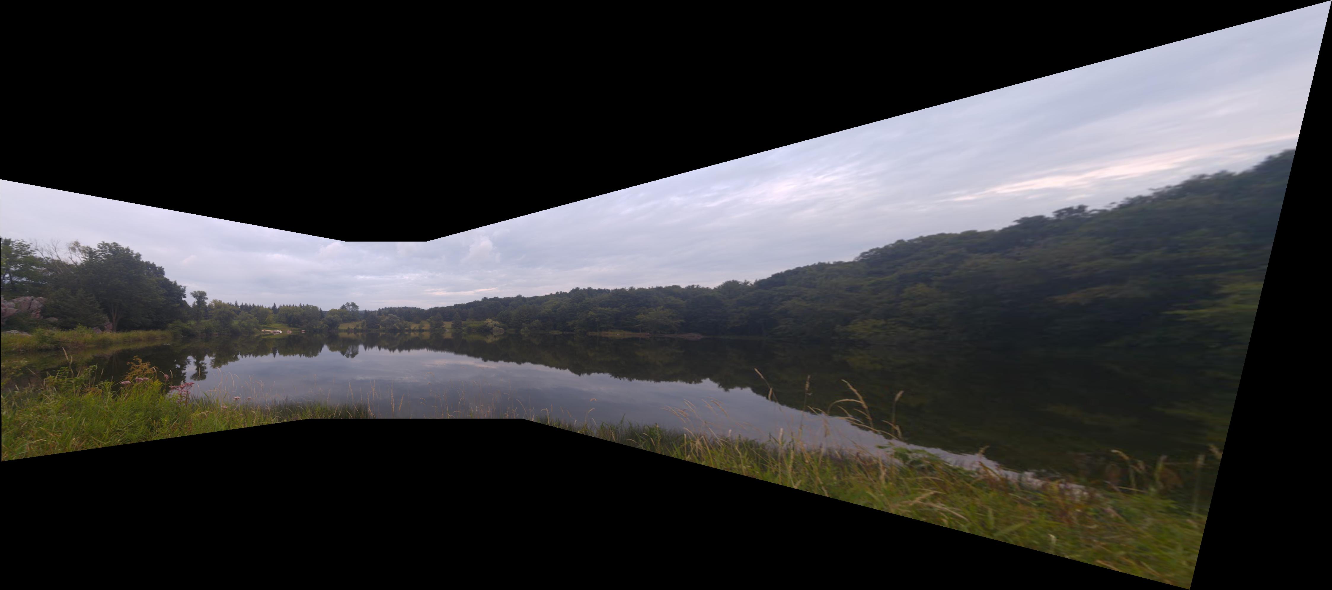
Lake in Wisconsin
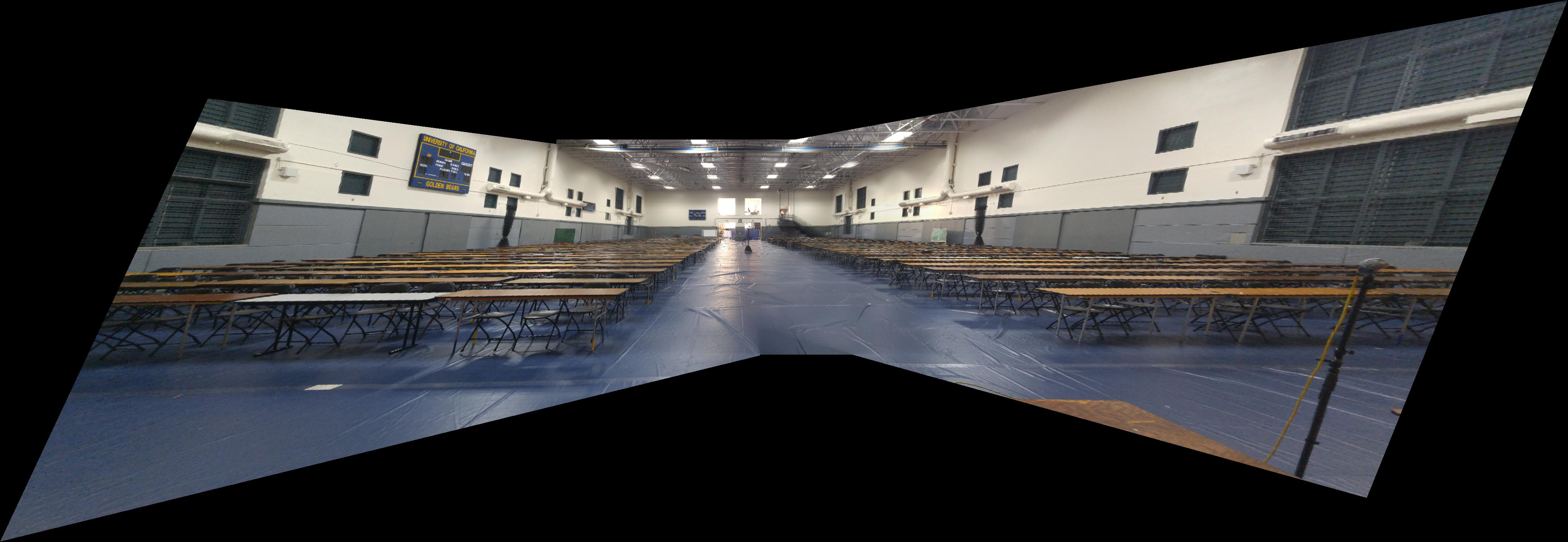
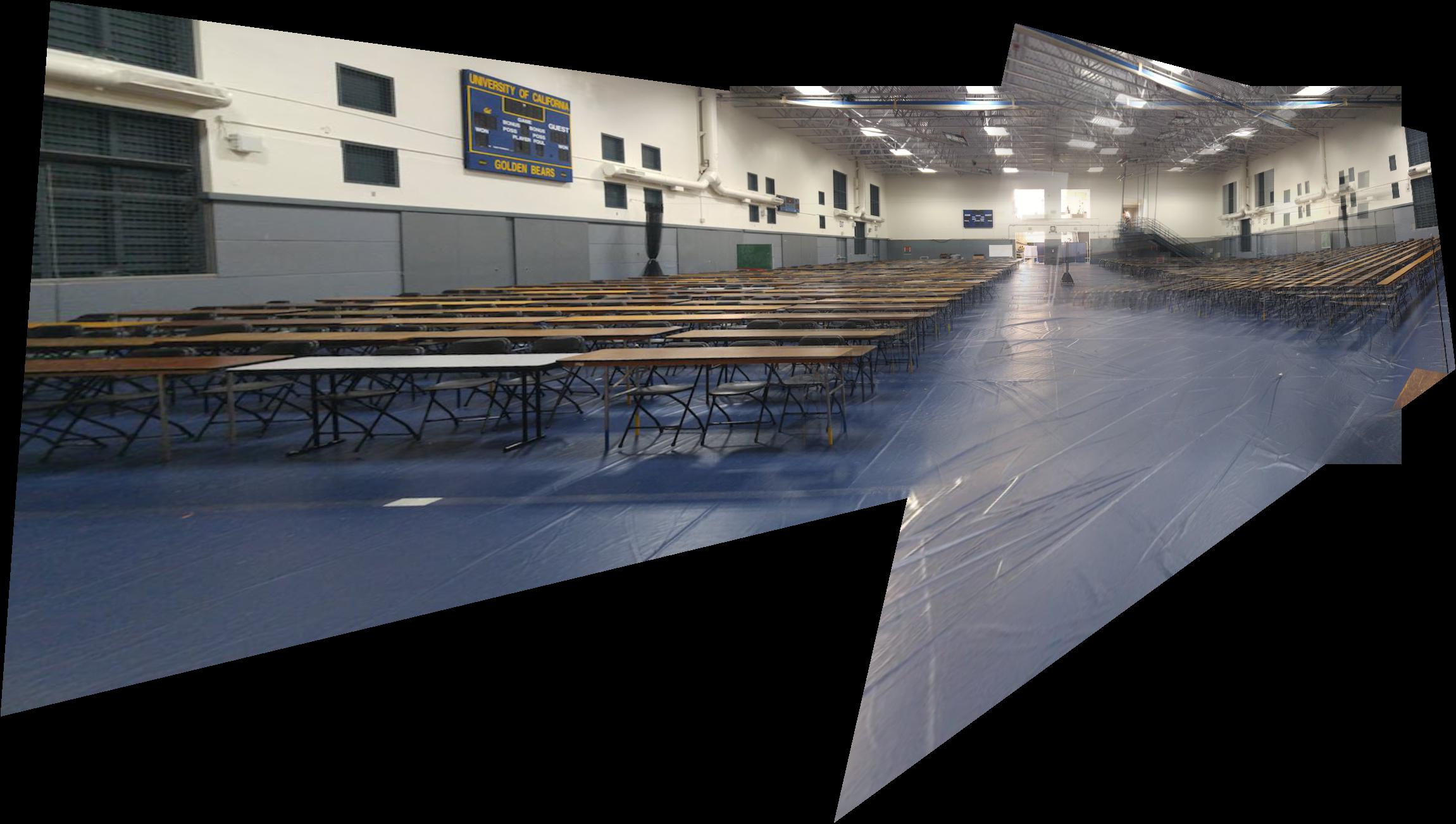
RSF Fieldhouse
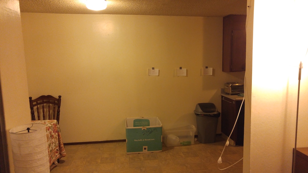
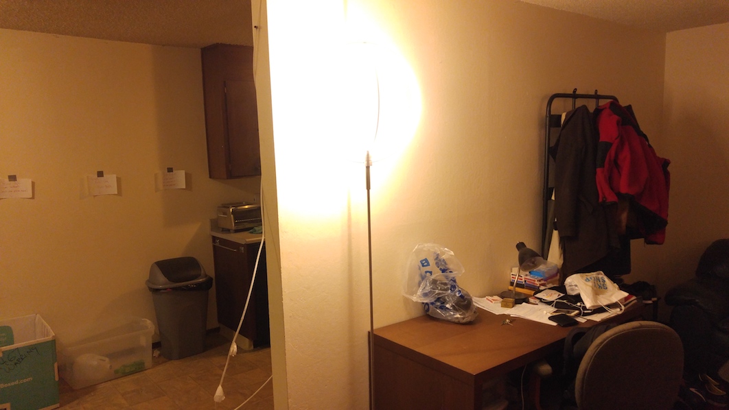
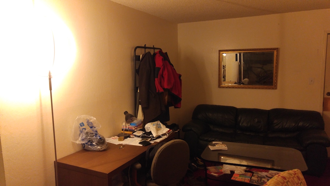
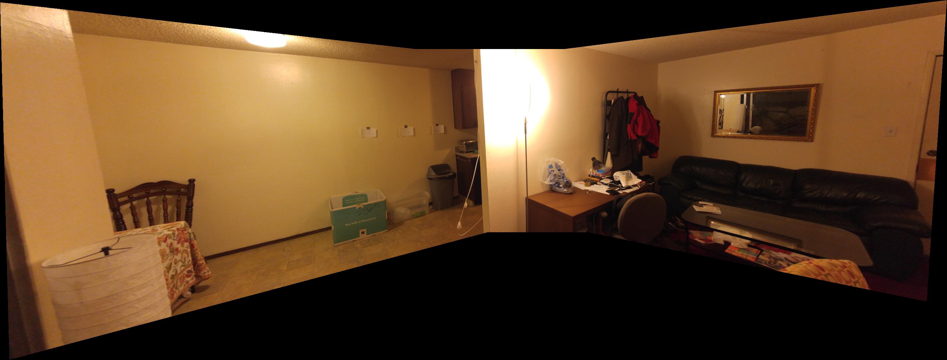
Living Room
The Lake and Living Room panoramas worked out very well. The transformation was
slightly different (evident if you look around the edges), but it seems
to have blended just as well (perhaps better?) than the manual ones.
The RSF one, however, did not work out very well. The middle and left images
have some ghosting effects (probably because they didn't match up completely--
maybe I translated the camera too much when I was taking the pictures... these
pictures weren't taken with this project in mind). The right image is just
completely off. I'm not exactly sure why this was -- perhaps feature matching
didn't quite work as expected, and there was too much noise in returned features,
perhaps even overpowering the regularization that RANSAC was supposed to provide.