[Auto]Stitching Photo Mosaics

CS194-26 Fall 2018

Andrew Campbell, cs194-26-adf

Part 1: Image Warping and Mosaicing

Introduction

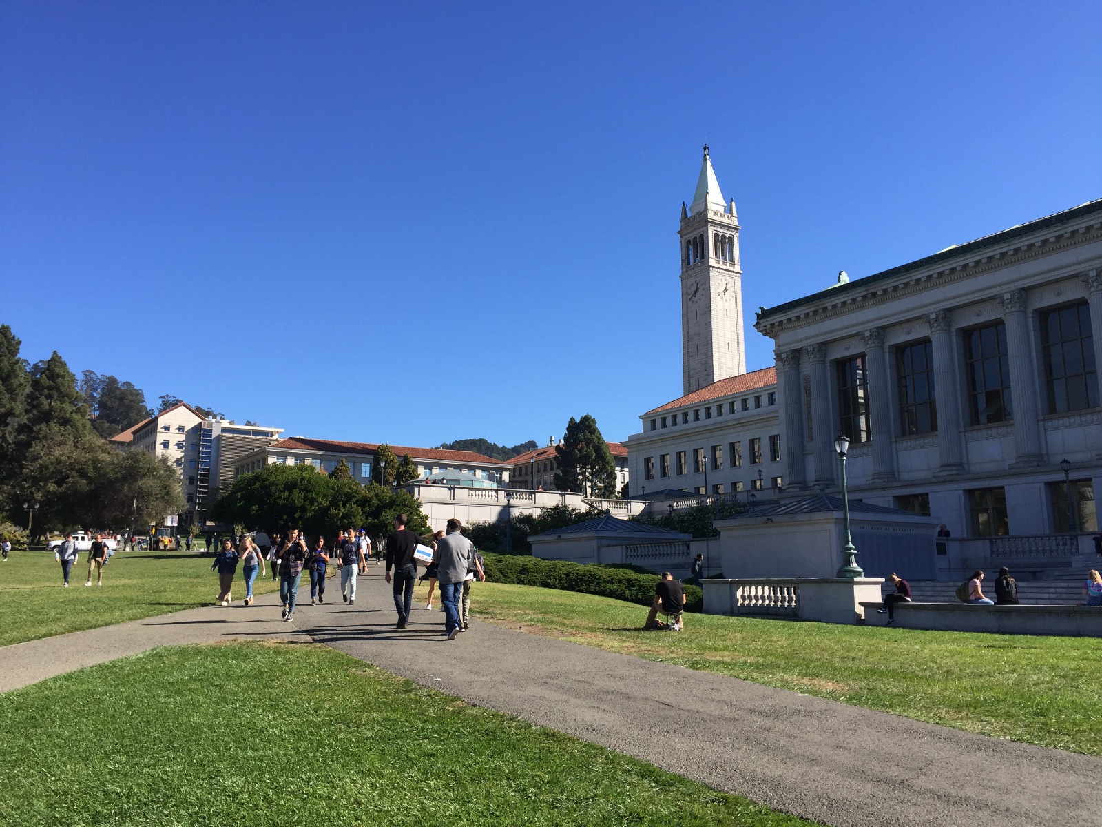
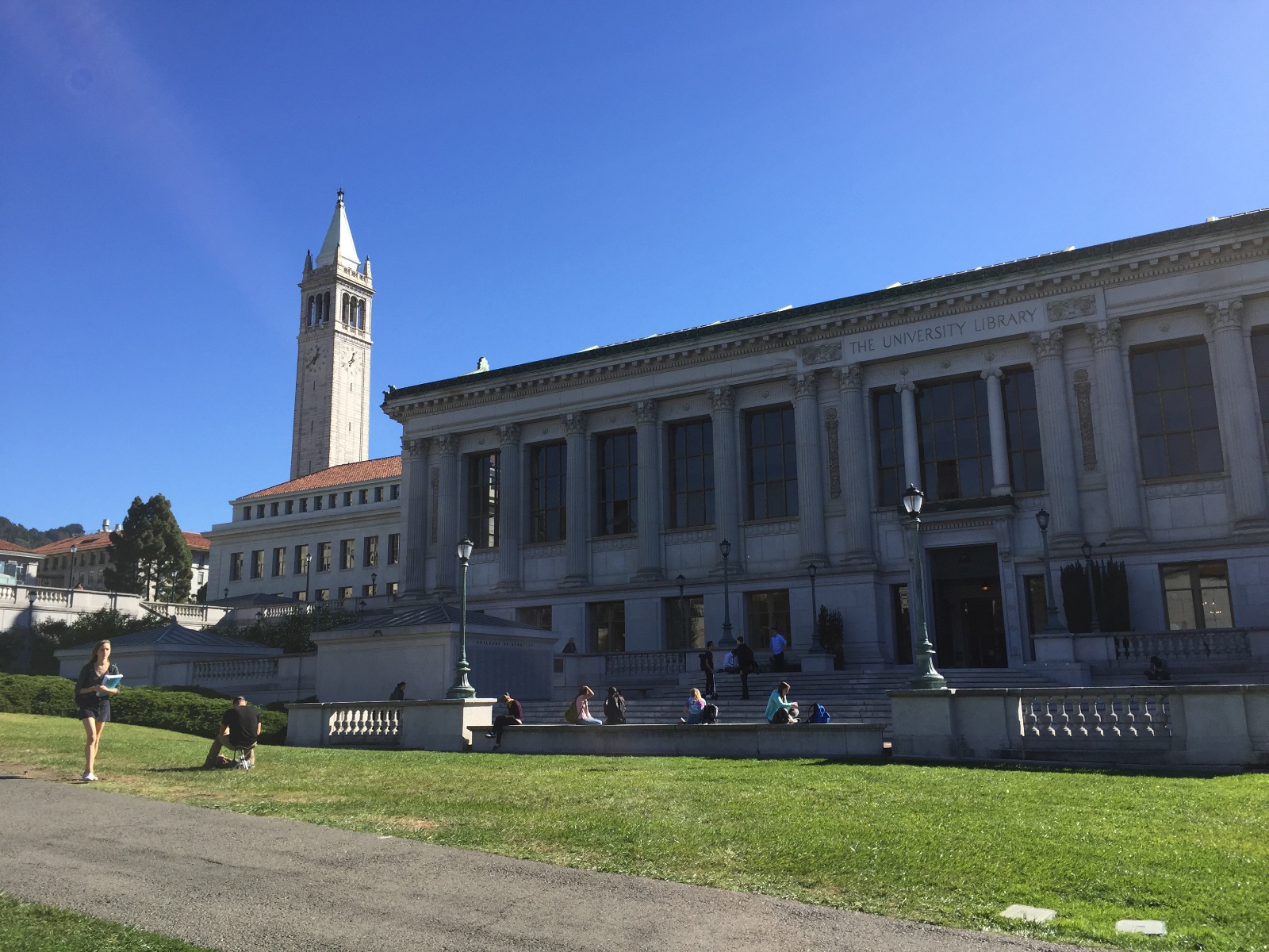
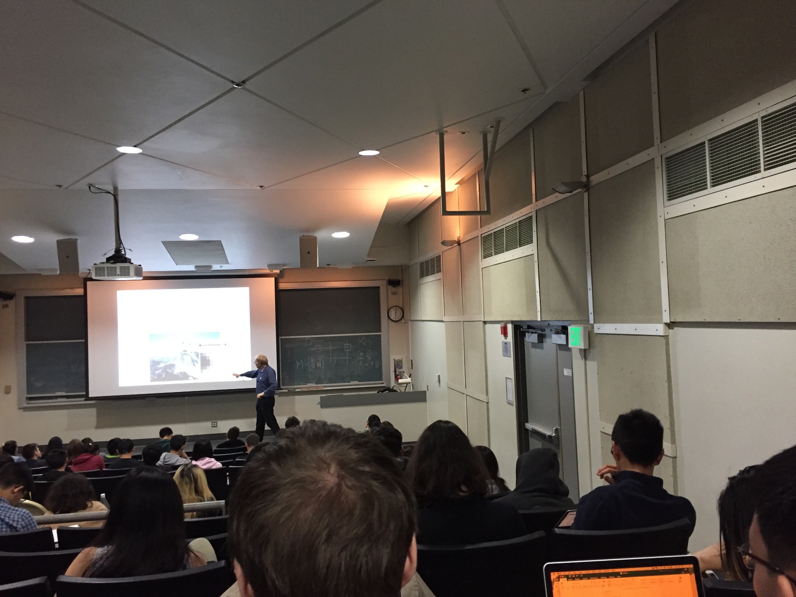
A panorama is a wide-angle view of a space. The most common method for producing panoramic images is to take a series of pictures with slightly overlapping fields of view and stitch them together. There are three main projection modes used in stiching images: spherical, cylindrical, and perspective. In this project, we will use perspective projection to project the panorama as though it were mapped on a flat surface.

Specifically, we will take as input three photos with the same point of view but with rotated viewing directions and with overlapping fields of view. Then we will use point correspondences to recover homographies from the left and center images and center and right images. We then perform a projective warp on the left and right images. Finally, we blend them together to create a panorama.

Recovering Homographies

Any two images of the same planar surface in space are related by a homography. The 3 x 3 homography matrix has the following form:

$$H = \begin{bmatrix} a & b & c \\ d & e & f \\ g & h & 1 \end{bmatrix}$$

It has eight degrees of freedom (as the last entry is fixed to be 1) and thus in principle only requires four point correspondence pairs to be recovered. However, this approach is prone to noise and in practice we find least square regression on many pairs of points works better. Given $n$ pairs of points for the first image $\left\{ (x_{1,i}, y_{1,i}) \right\}_{i=1}^{n}$ and second image $\left\{ (x_{2,i}, y_{2,i}) \right\}_{i=1}^{n}$, we wish to find $H$ such that

$$\sum_{i=1}^{n} \lVert H \begin{bmatrix} x_{1,i} \\ y_{1,i} \\ 1 \end{bmatrix} - \begin{bmatrix} wx_{2,i} \\ wy_{2,i} \\ w \end{bmatrix} \rVert_2^2$$

is minimized. It can be shown through some algebra that the relevant matrix equation $Ax=b$ is

$$\begin{bmatrix} x_{1,1} & y_{1,1} & 1 & 0 & 0 & 0 & -x_{1,1} x_{2,1} & -y_{1,1} x_{2,1} \\ 0 & 0 & 0 & x_{1,1} & y_{1,1} & 1 & -x_{1,1} y_{2,1} & -y_{1,1} y_{2,1} \\ & & & & \vdots & & & \\ x_{1,n} & y_{1,n} & 1 & 0 & 0 & 0 & -x_{1,n} x_{2,n} & -y_{1,n} x_{2,n} \\ 0 & 0 & 0 & x_{1,n} & y_{1,n} & 1 & -x_{1,n} y_{2,n} & -y_{1,n} y_{2,n} \\ \end{bmatrix} \begin{bmatrix} a \\ b \\ c \\ d \\ e \\ f \\ g \\ h \end{bmatrix} = \begin{bmatrix} x_{2,1} \\ y_{2,1} \\ \vdots \\ x_{2,n} \\ y_{2,n} \end{bmatrix}.$$

We can solve for $x$ using least squares to recover $H$.

To obtain point correspondences, we manually record coordinates of the same features in both images. This is a tedious task; we will automate the process in the next part. I found that using 20 point correspondences was sufficient.

Image Rectification

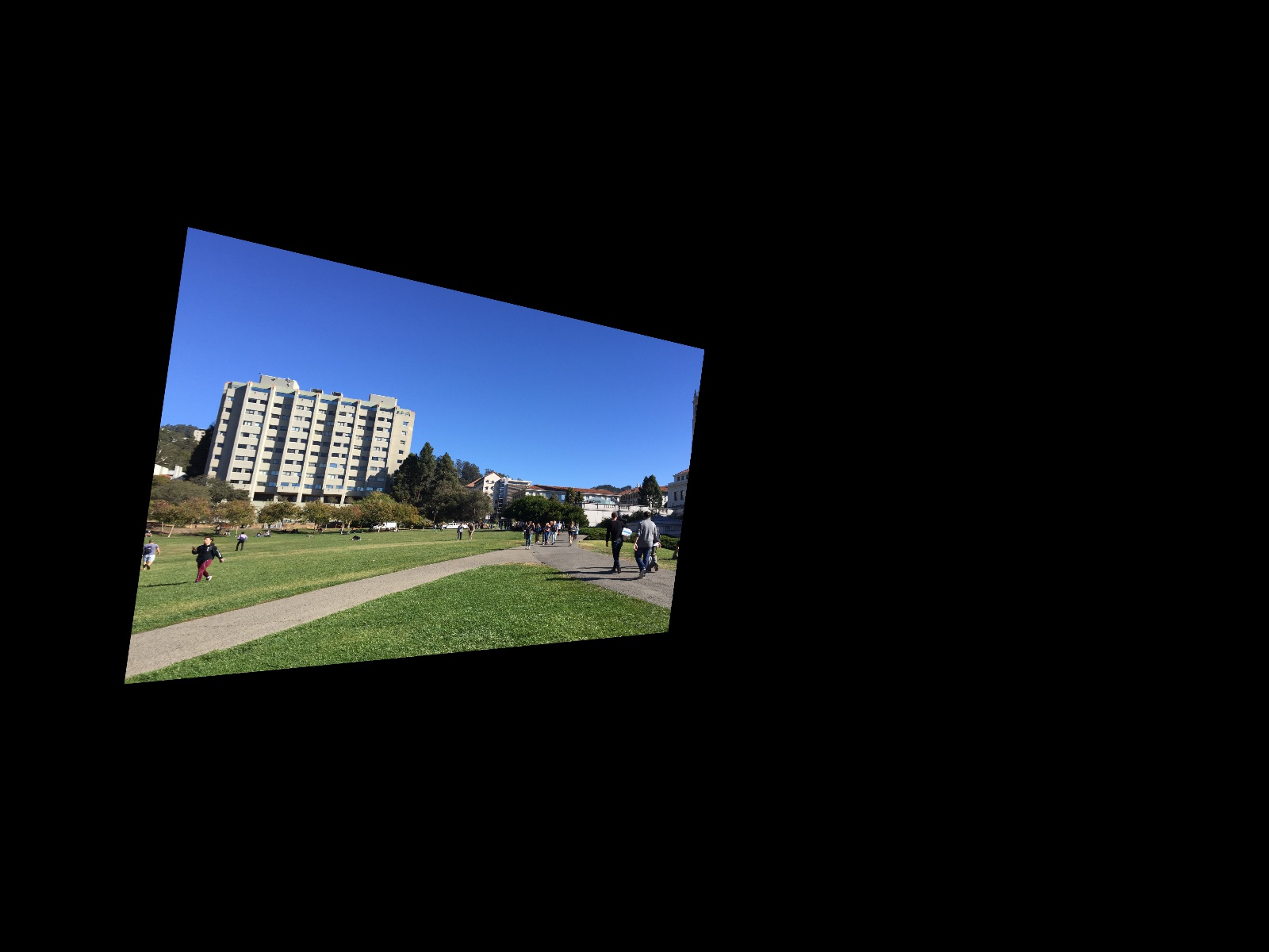
We can now perform (inverse) image warping: for every coordinate value in the output result, multiply by the (inverse) homography matrix, taking care to normalize $w$ to be $1$, to recover the “lookup” coordinates in the original image. We perform interpolation to avoid aliasing.

One application of a homography is image rectification: given an image containing a planar surface, warp it so that it is frontal-parallel. We simply select 4 points representing the corners of the plane in the original image and choose the correponding points in the output to be the corners of a rectangle. Below we illustrate some examples.

---

Mosaics

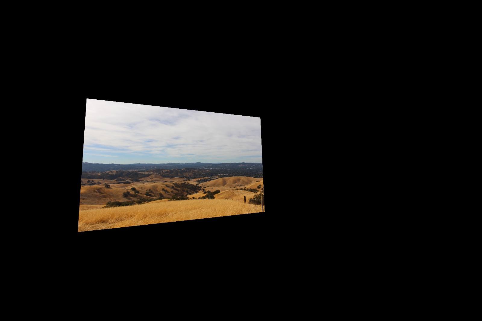
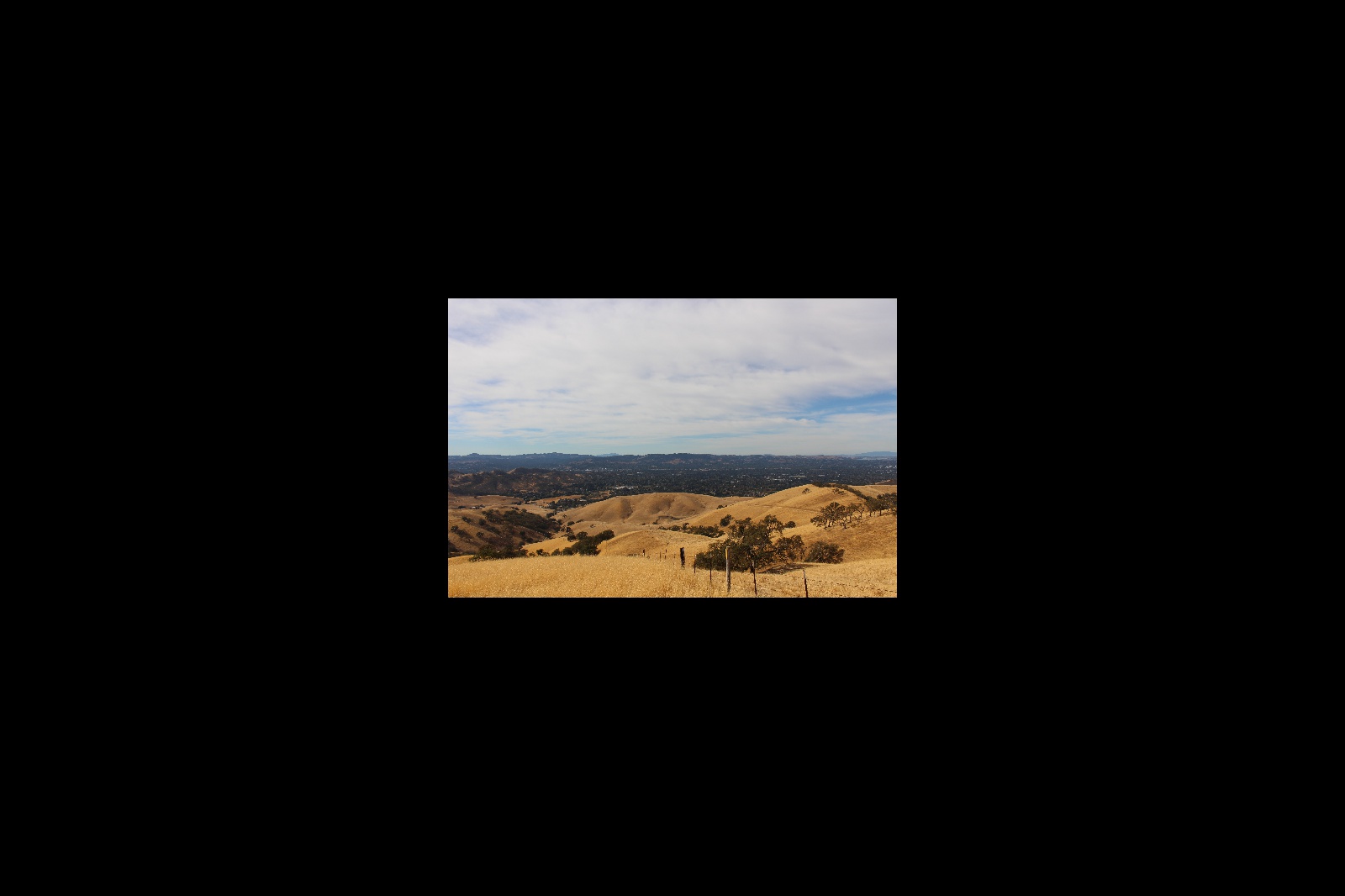
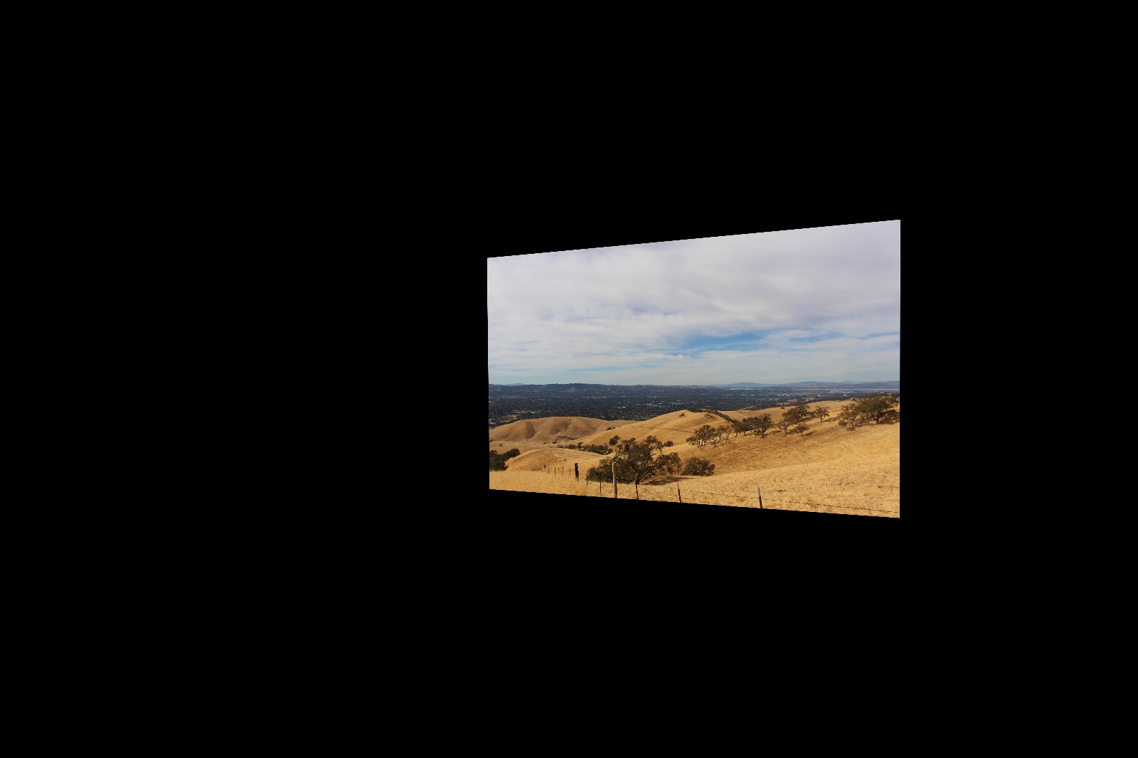
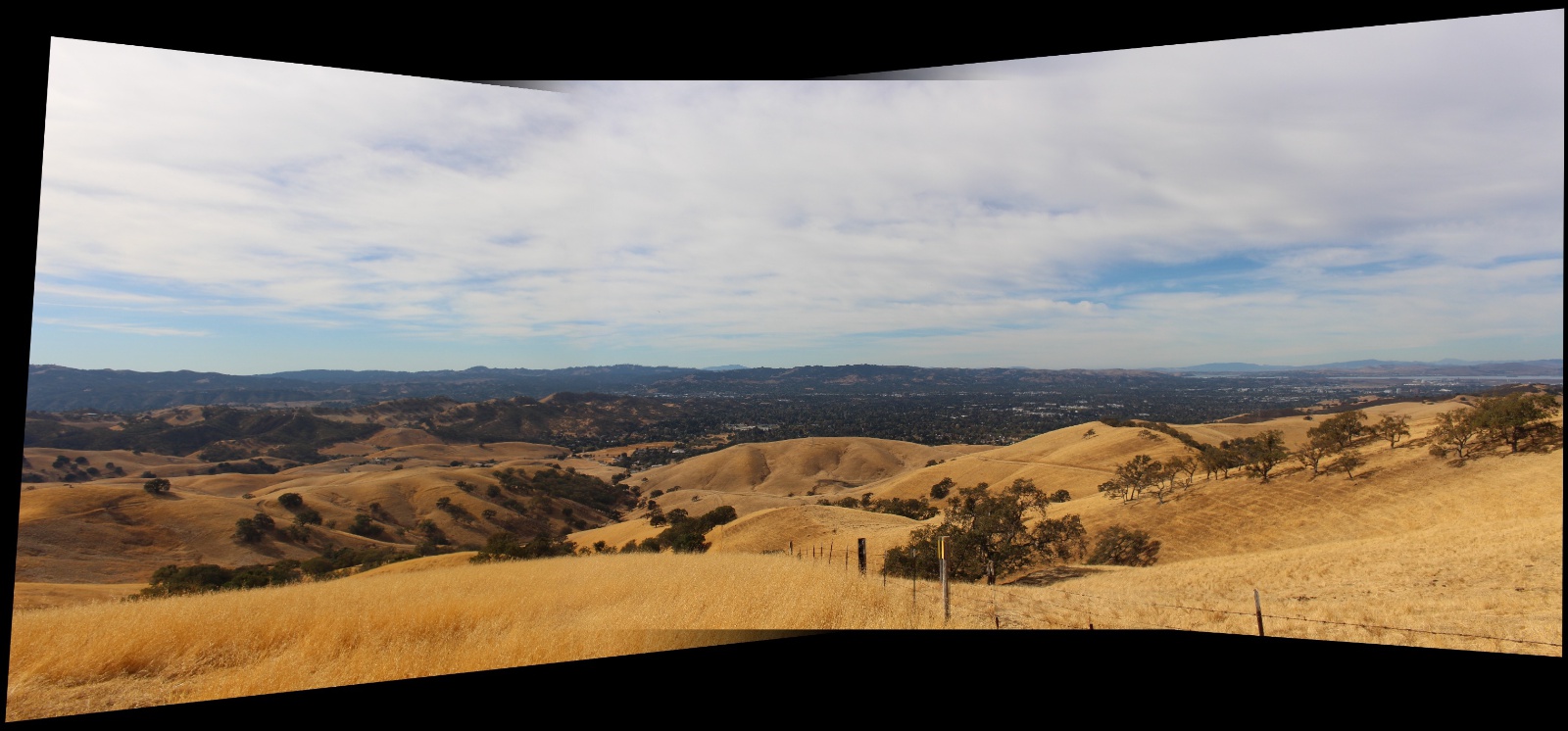
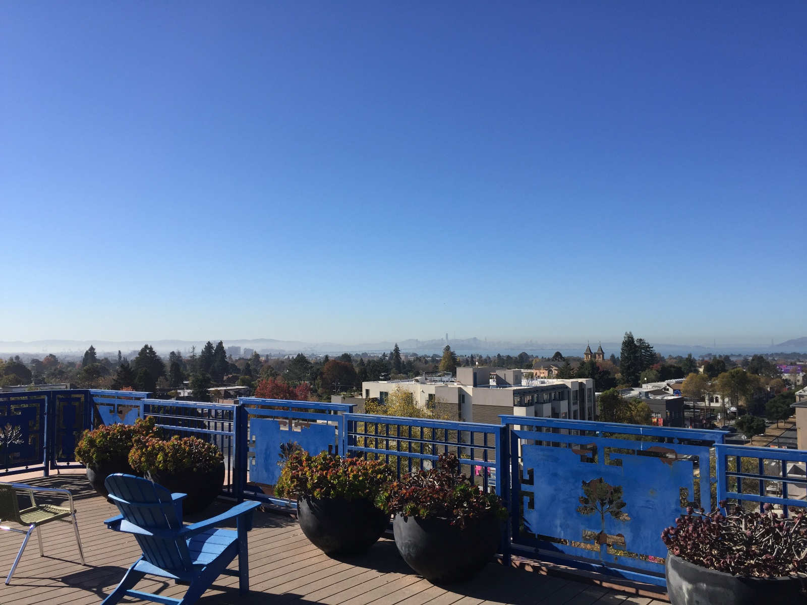
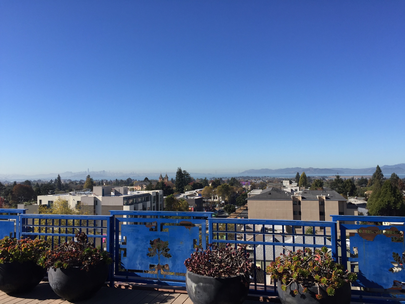
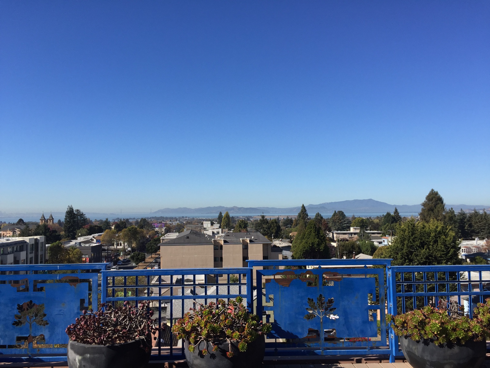
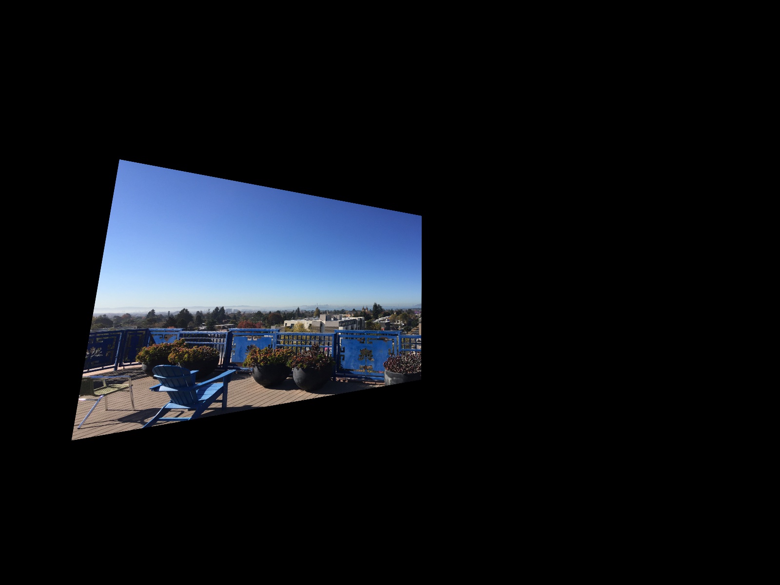
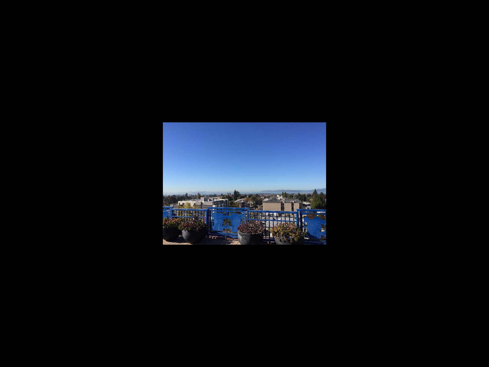
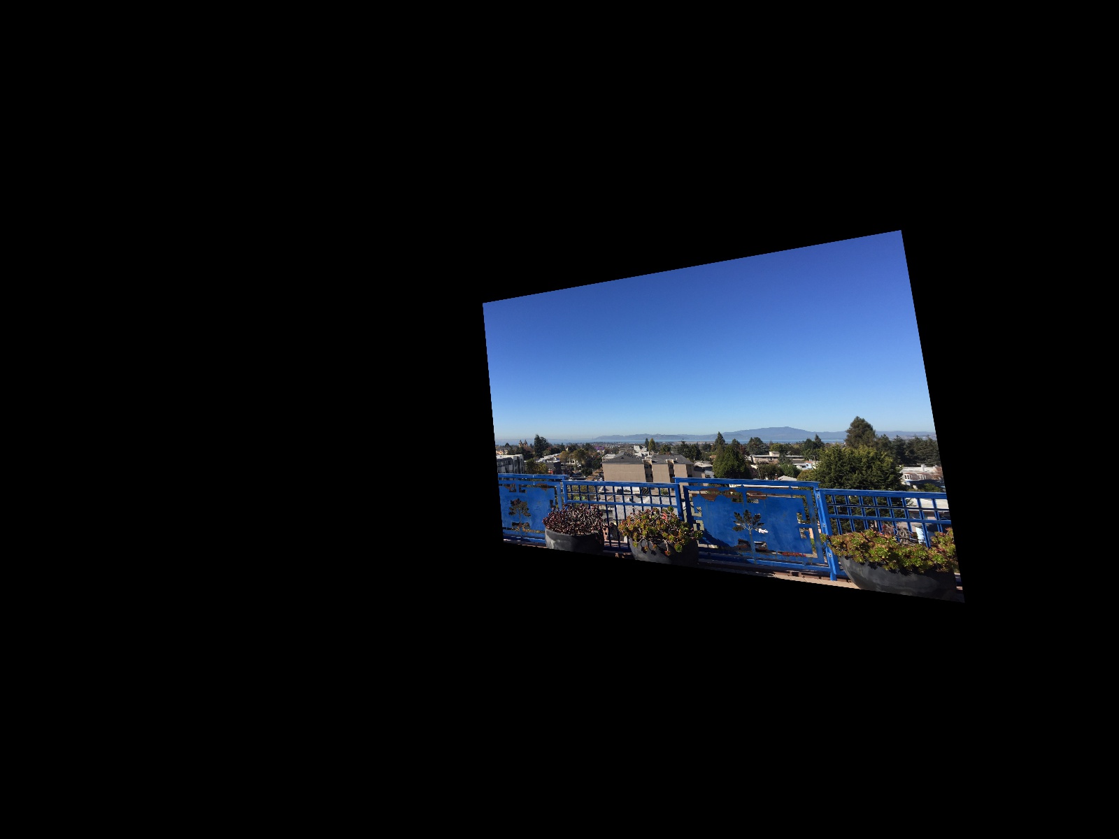
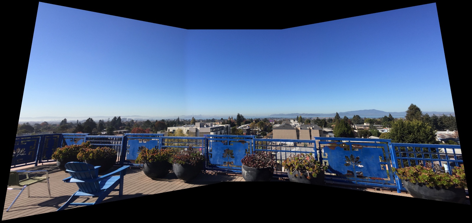
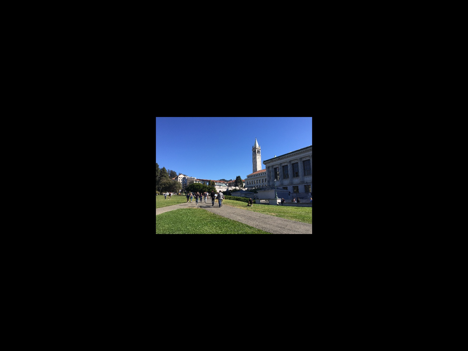
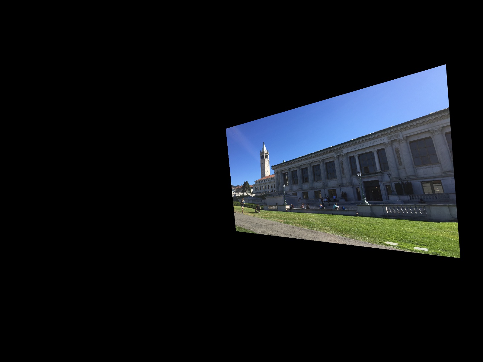
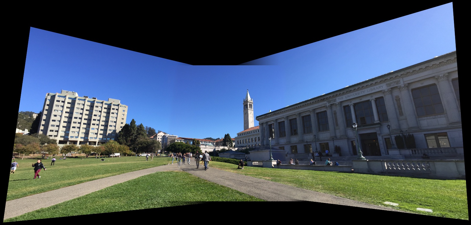
Given three images with the same point of view but with rotated viewing angles and overlapping fields of view, we can create a mosaic. We can recover the homography transformation as detailed above, and warp the left and right images appropriately. Note that in order to capture all of the warped result, we first create a large blank canvas and place the image in the center.

In order to blend the resulting warps, we can simply use alpha blending by multiplying the image by a feathered mask. Some example masks for the left, center, and right images, respectively, are shown below.

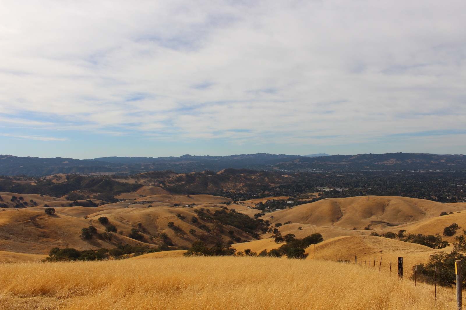
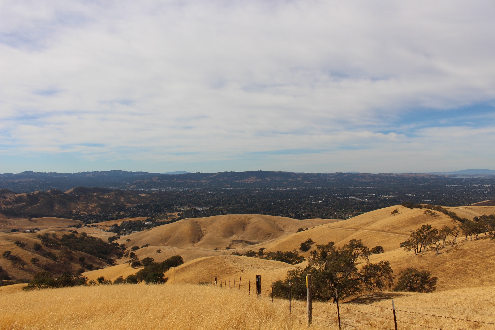
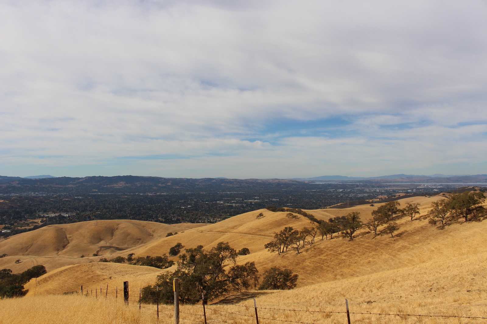
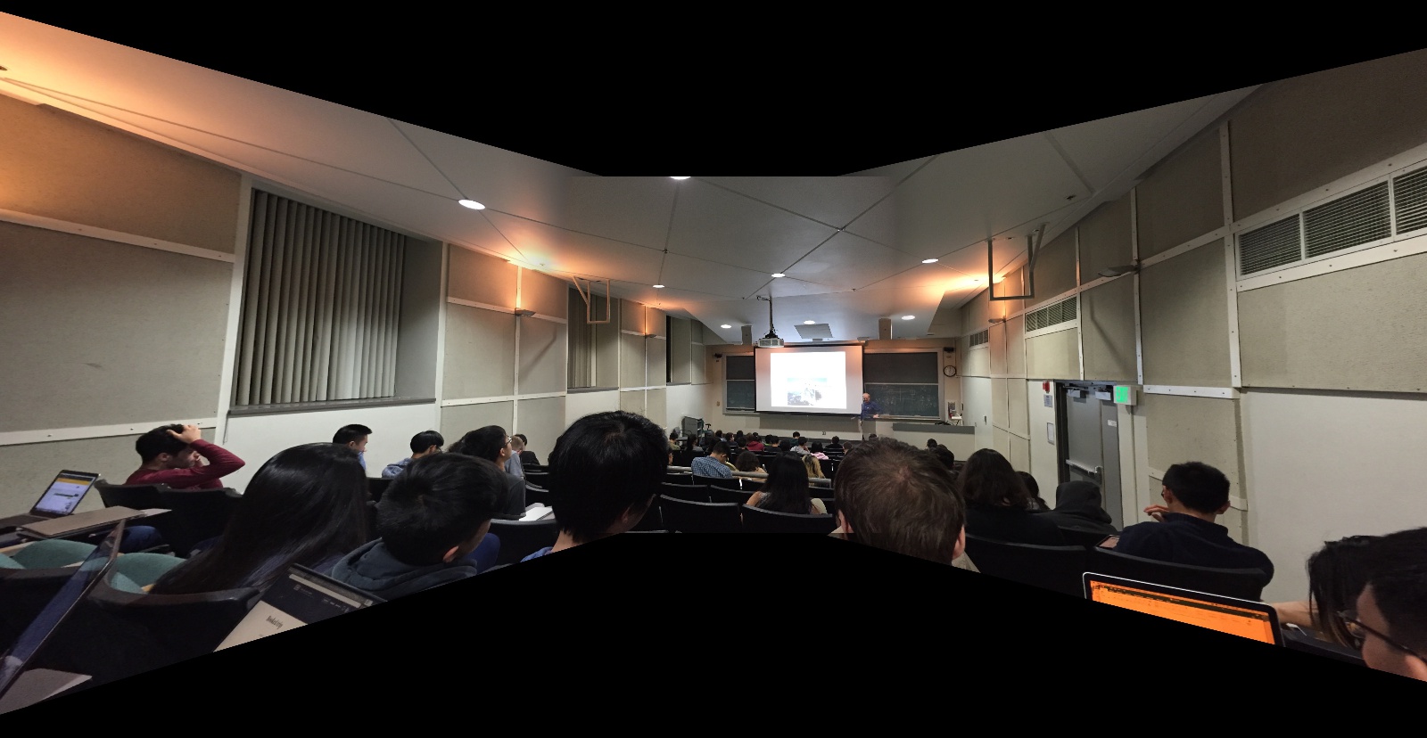
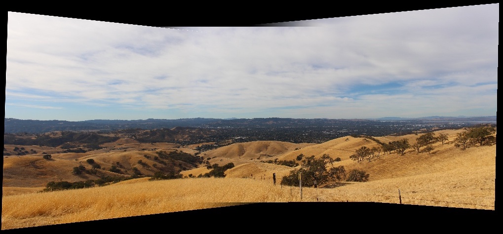
Results

---

---

---

---

Part 2: Automatic Stitching

Manually picking point correspondences is a tedious task. We will use a (simplified) implementation of Multi-Image Matching using Multi-Scale Oriented Patches to automate this process.

Harris Corners

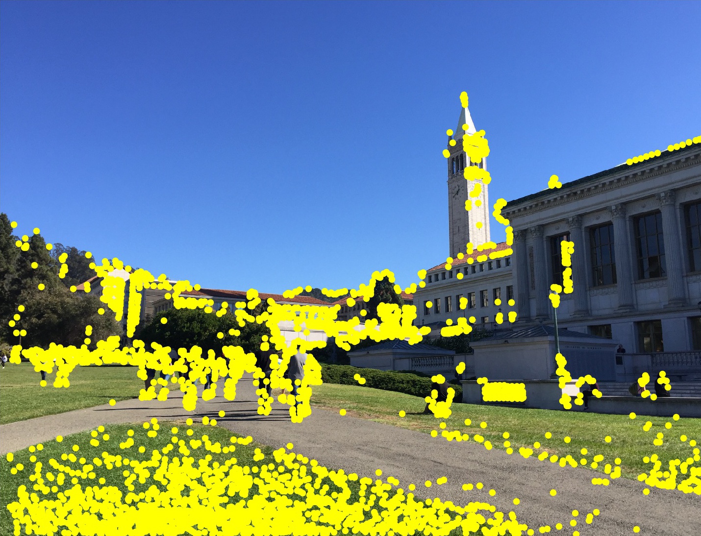
The first step in finding matches between images is to generate potential points of interest in the images. The Harris Corner Detector is an algorithm appropriate for this task; it finds corners in an image, or points whose local neighborhoods stand in two different edge directions. I used the corner_harris and corner_peaks functions from the skimage.feature library to do the work here (I found that peak_local_max resulted in far too many random points). corner_harris returns a response matrix representing the corner strength at every pixel coordinate in the image, which will be useful later.

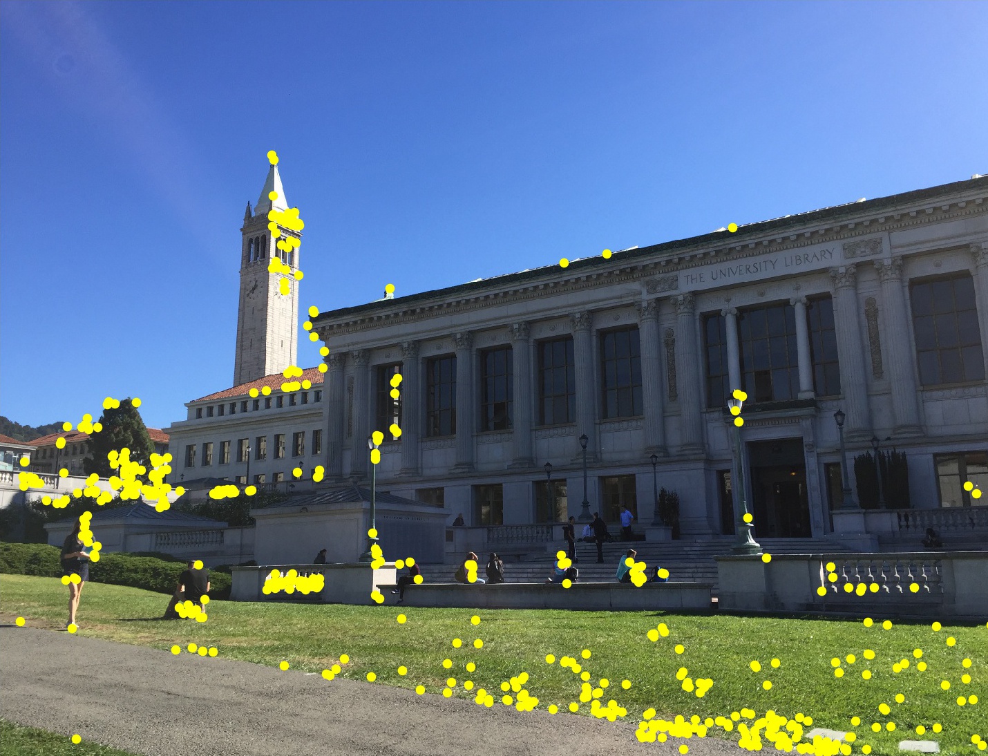
Shown below are two images with their Harris corners overlaid in yellow.

Adaptive Non-Maximal Suppression

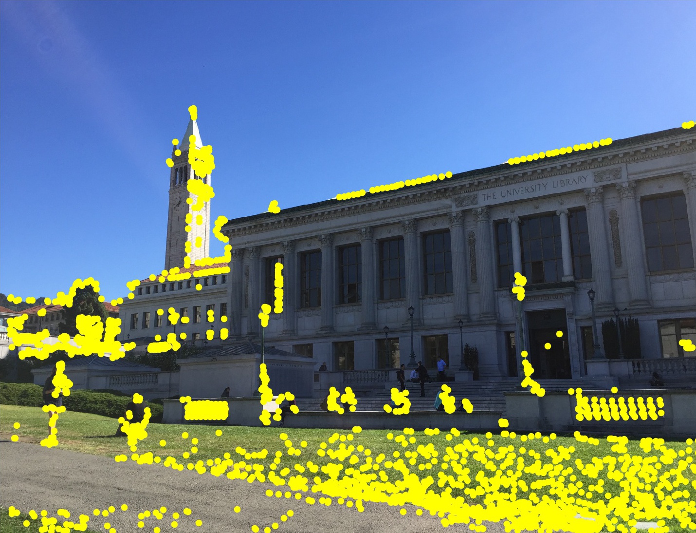
As we can see, there are a lot of Harris corners found. The computational cost of matching is superlinear in the number of interest points, so it is desirable to limit the maximum number of interest points extracted from each image. At the same time, it is important that interest points are spatially well distributed over the image. The algorithm presented in the paper, Adaptive Non-Maximal Suppression or ANMS, solves this problem by selecting the points with the largest values of $r_i$, where $r_i$ is the minimum suppression radius of point $x_i$:

$$r_i = \min_{j} | x_i - x_j |, \text{s.t. }f(x_i) < c_{\text{robust}} f(x_j), x_j \in \mathcal{I}$$

Here, $\mathcal{I}$ is the set of all interest points and $f(x_j)$ represents the corner response of point $x_j$ (which we get from response matrix we retained from the previous step).

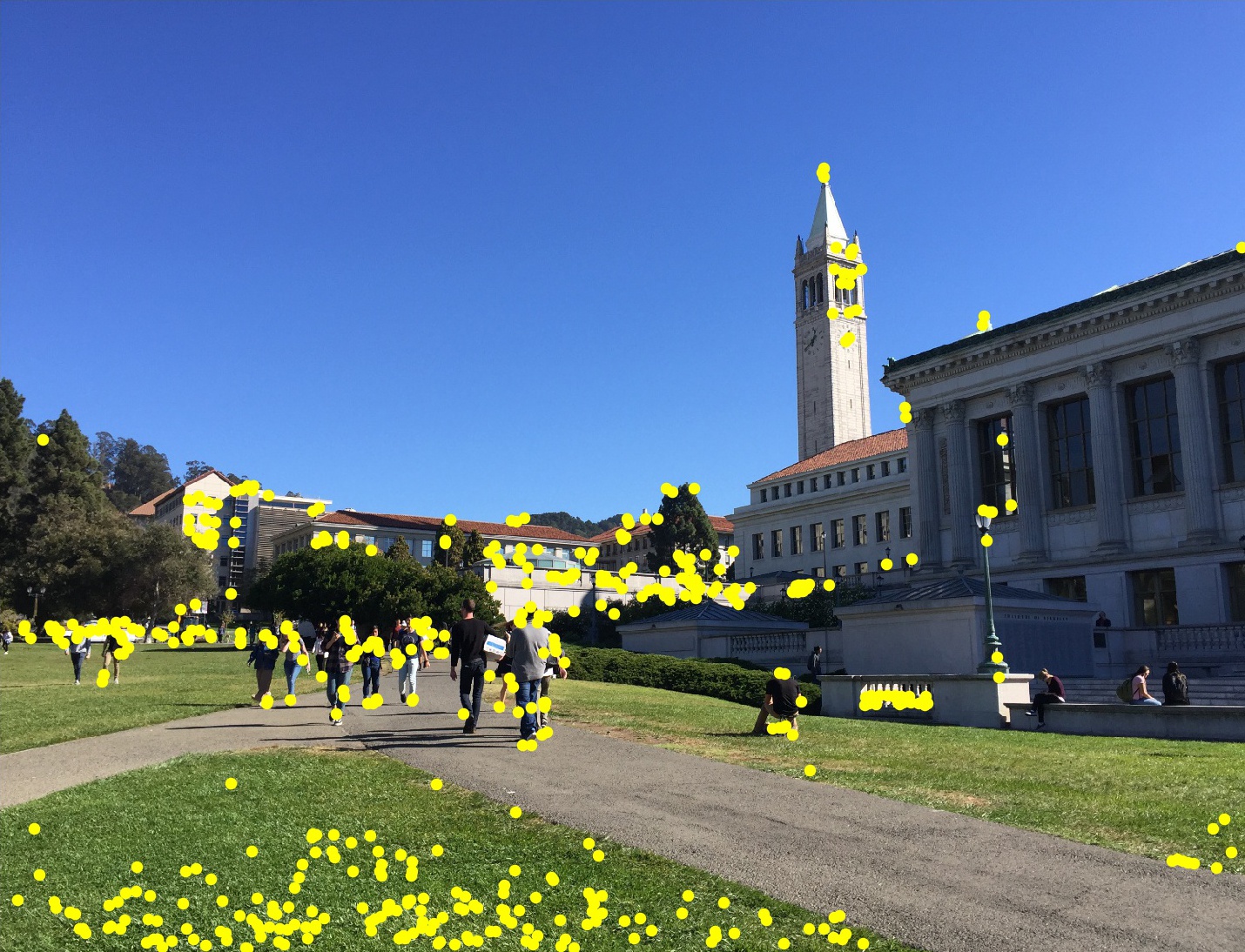
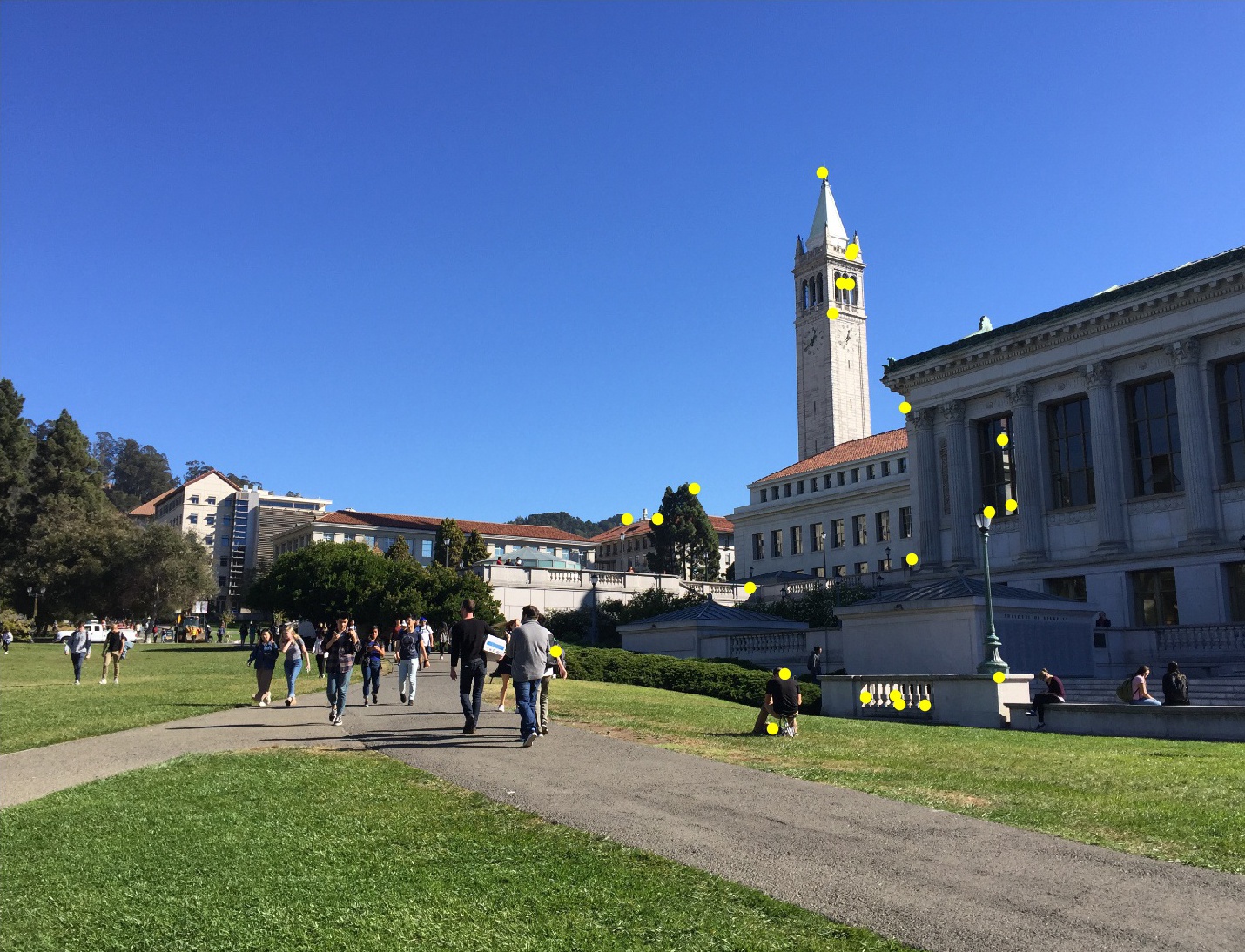
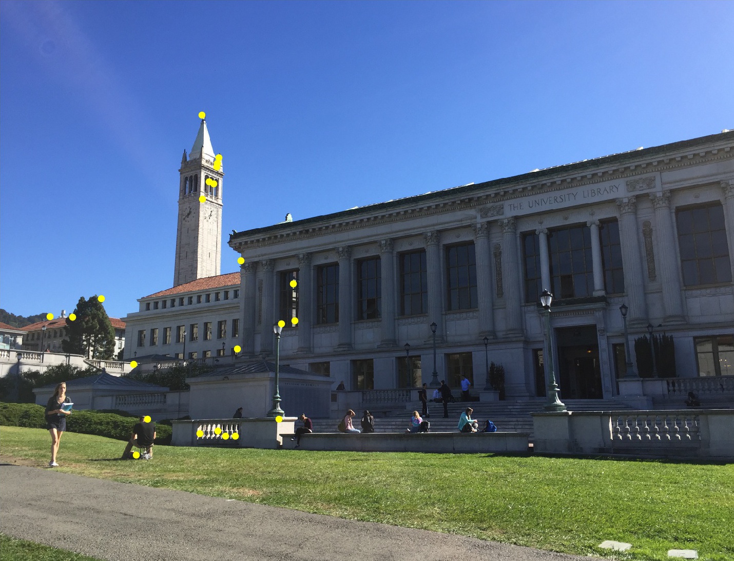
In simpler terms, for each point, we find the minimum radius to the next point such that the corner response for the existing point is less than some constant multiplied by the response for the other point. Using $c_{\text{robust}} = 0.9$ and keeping only the top 500 points, the corners left are shown below.

Feature Descriptor Extraction

We can now use our interest points as feature descriptors. We do this by extracting a 40x40 patch centered about each point and downsampling the patch to 8x8 - this is done to eliminate high frequency signals. We additionally bias/gain normalize the patches by subtracting the mean and dividing by the standard deviation. This makes the features invariant to affine changes in intensity (bias and gain).

Feature Matching

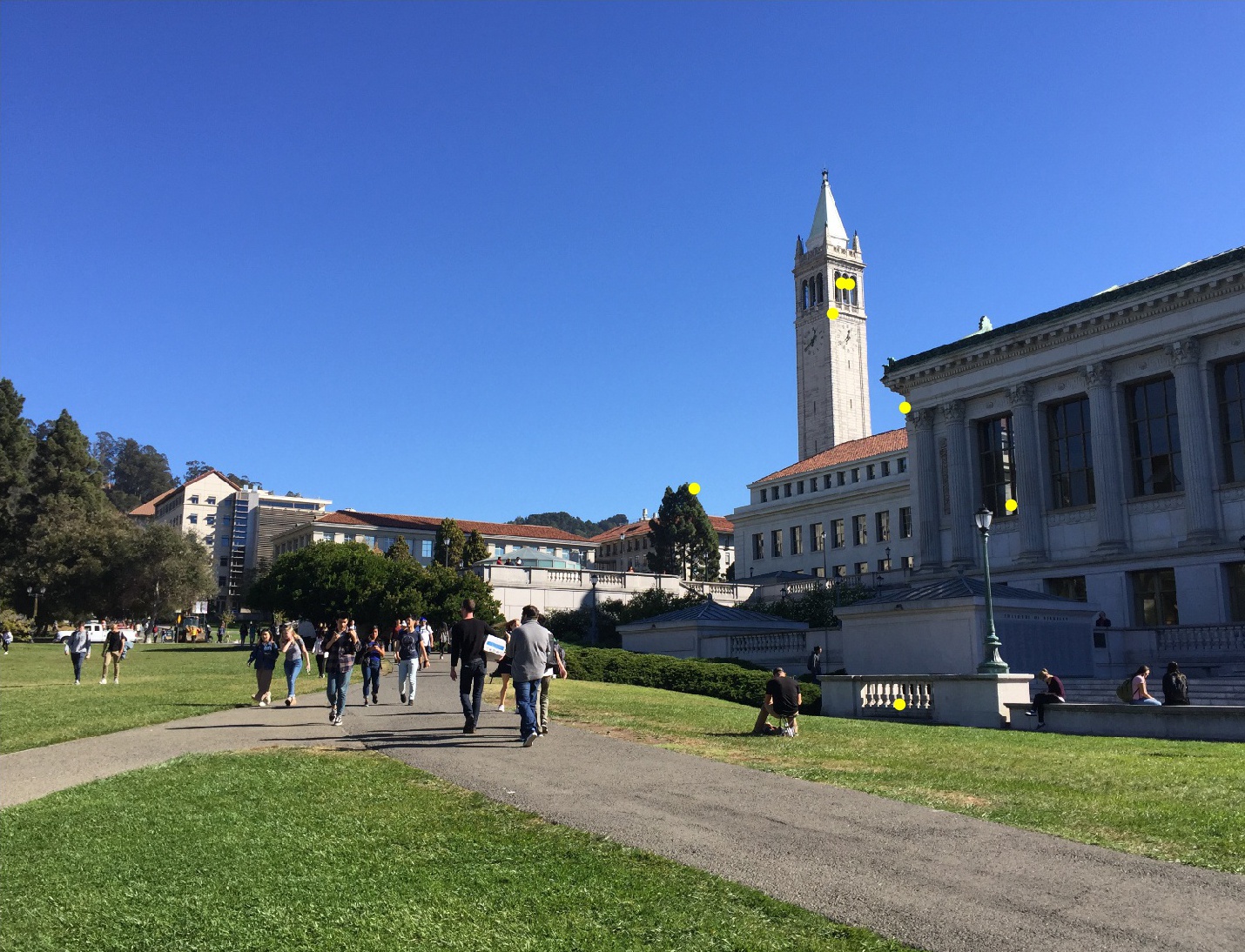
The next step is to find geometrically consistent feature matches between two images. First we vectorize the feature descriptors extracted in the last step. Then we compute the squared distance from every feature in the first image to every feature in the second image (essentially a nearest-neighbor search). We use the Lowe ratio test: if the ratio of the distance to the 1-NN over the distance to the 2-NN is less than some threshold, we consider the pair to be a match. The rationale is that true feature matches have a single good match, not multiple. I found that a threhold value of $0.6$ worked well. The matches are shown below.

RANSAC

The feature matches computed above look quite good, but there is a noticeable outlier in the left image. There is a feature point on the the pedestrian’s arm in the left image with no corresponding match in the right image. The least-squares homography calculation is highly sensitive to outliers, so we must reject them first. To that end, we use RANSAC, or random sample concensus. We choose 4 potential matches at random from the first image and compute an exact homography $H$. We then warp all of match points from the first image according to $H$ and compute the SSD error between them and the real match points in the second image. Define inliners to be the set of points whose error is less than some threshold. Repeating this process several times, we keep track of the largest set of inliners and retain them as our true feature matches.

I used an error threshold of $0.5$ and 100 iterations. The matches left after RANSAC are shown below.

As we can see, the outlier(s) have been discarded.

Having successfully recovered point correspondences automatically, we can now proceed as in Part 1 to stich the images together.

Results

Below we compare the (cropped) mosaics resulting from automatic feature matching (left) and manual feature feature mapping (right) from before.

I think the results are pretty comparable. The manual correspondence points look slightly beter, but it’s not a big deal.

---

Bells and Whistles

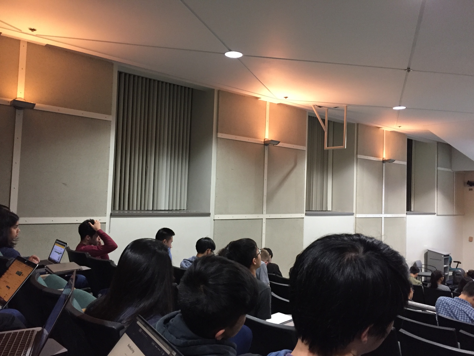
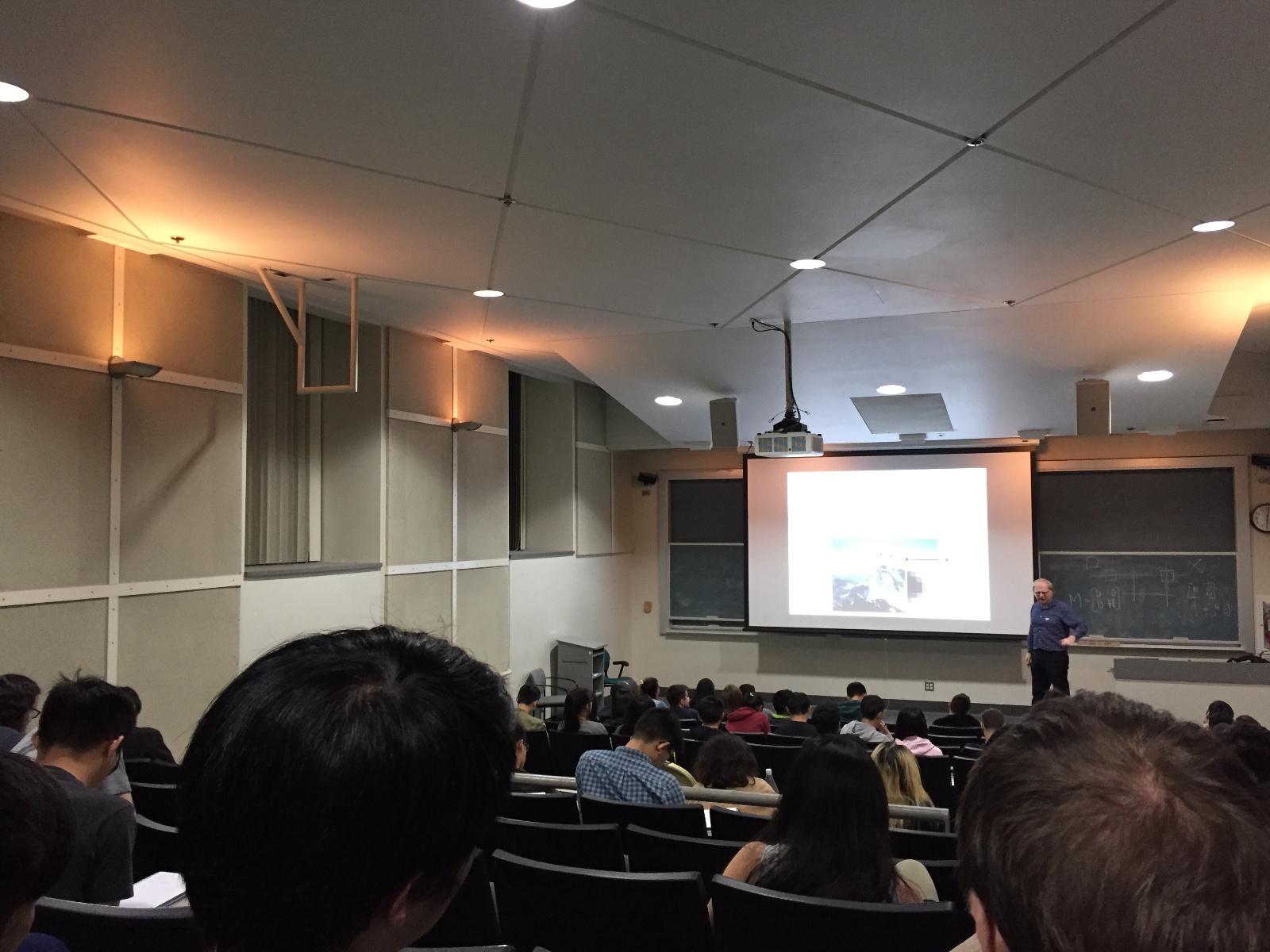
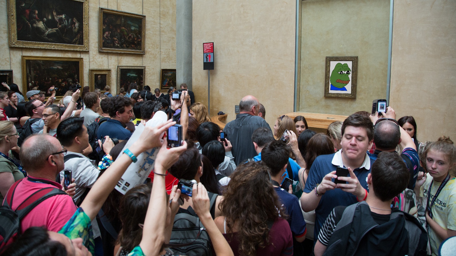
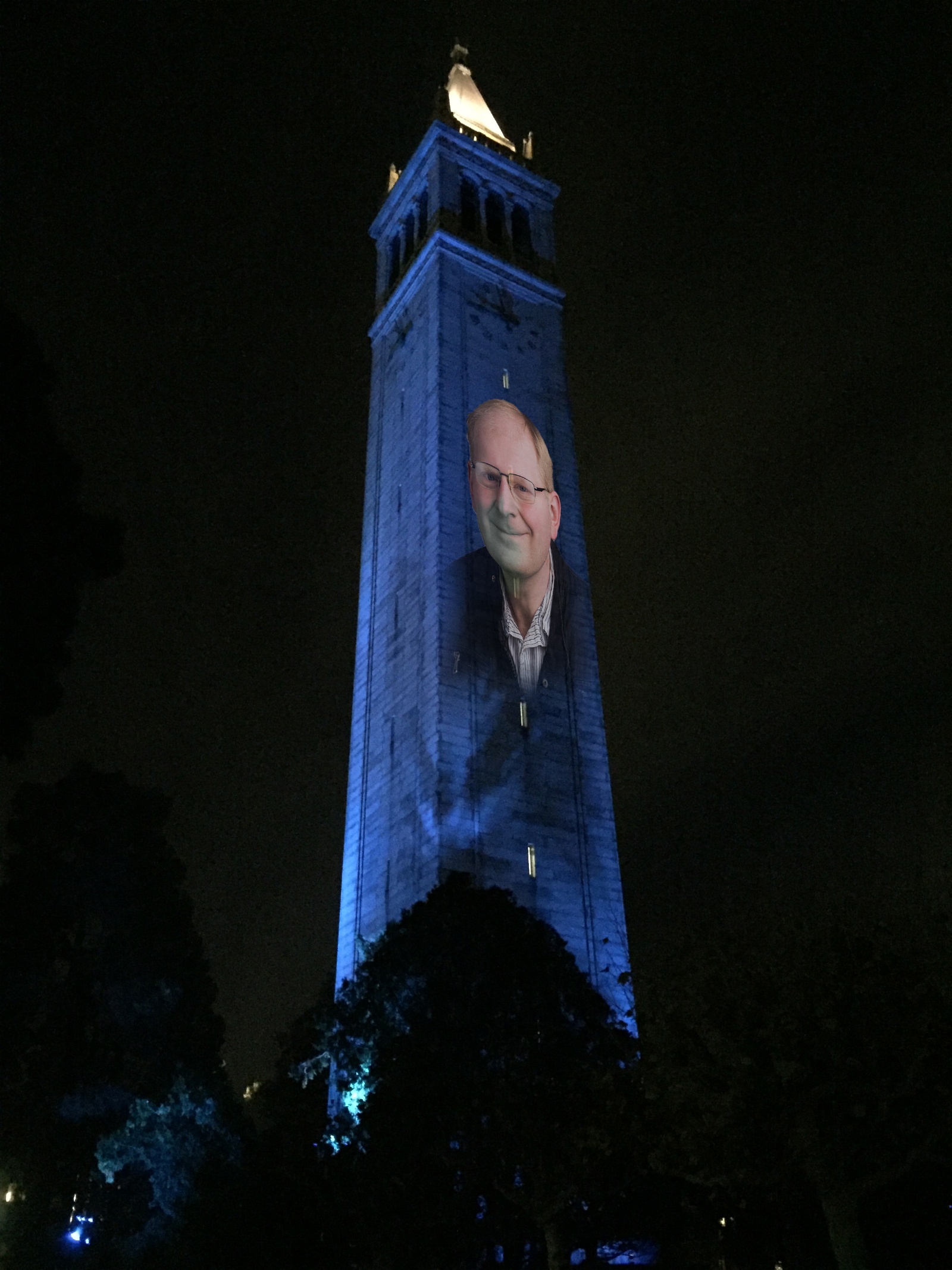
Warping and blending is good for more than just panoramas. Here are some images created by manually defining four-point correspondences.

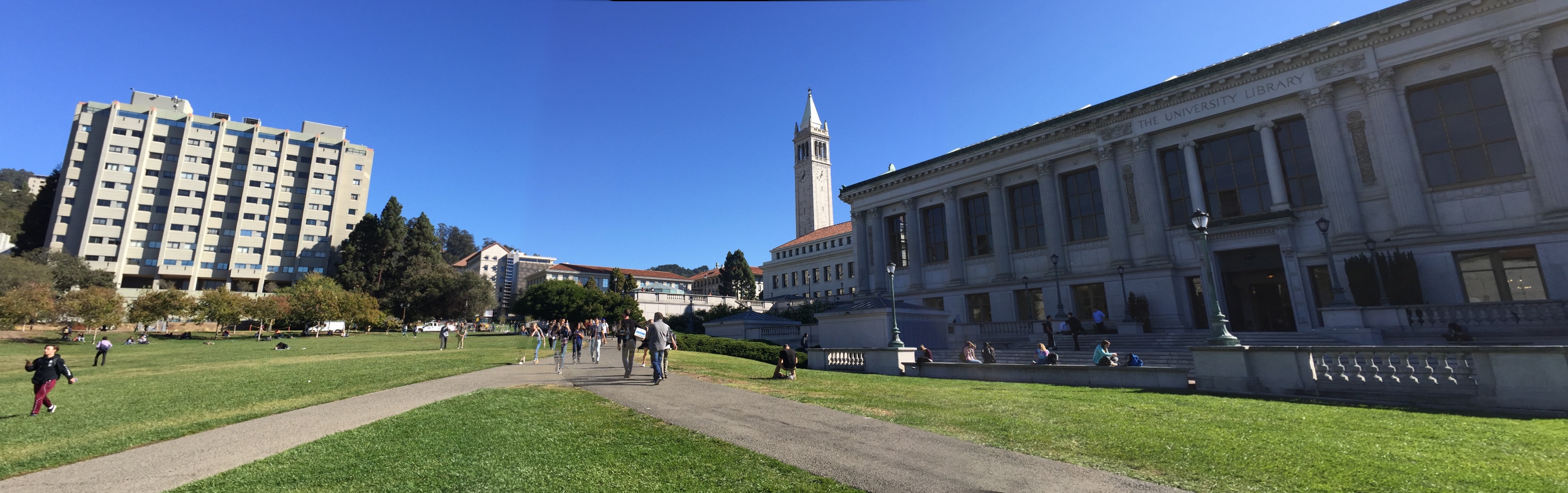
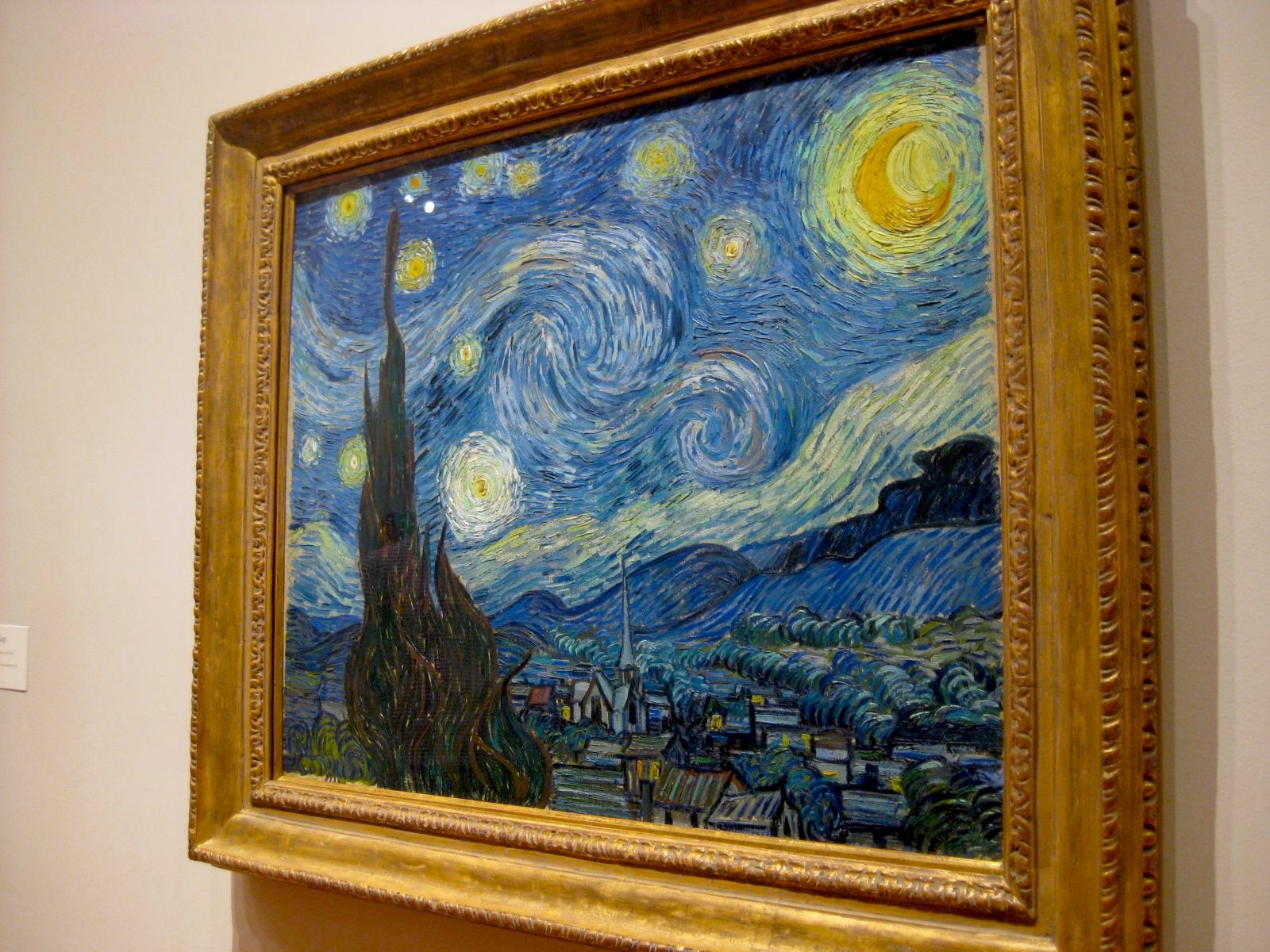
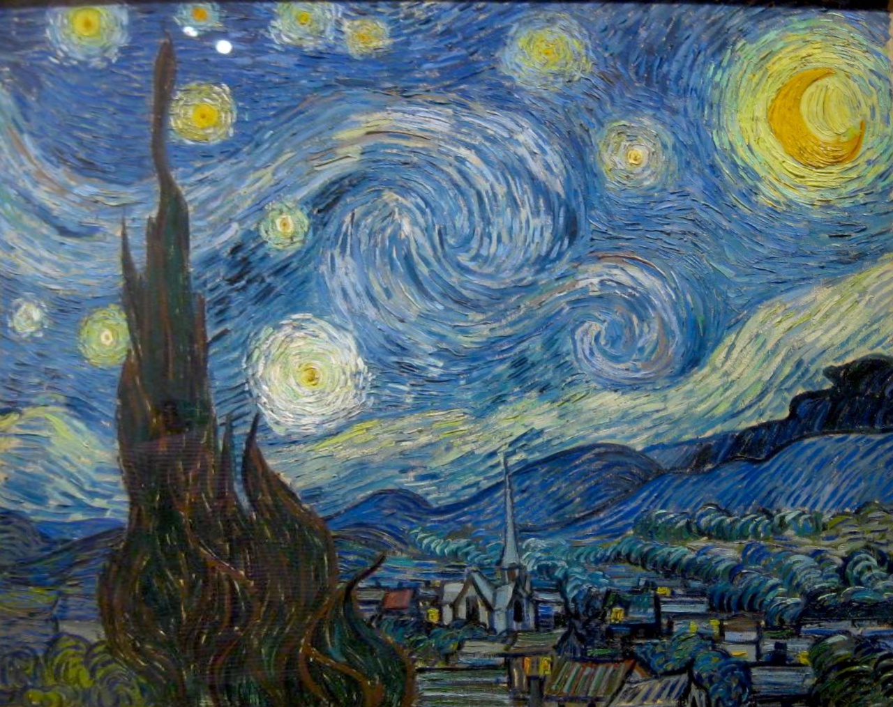
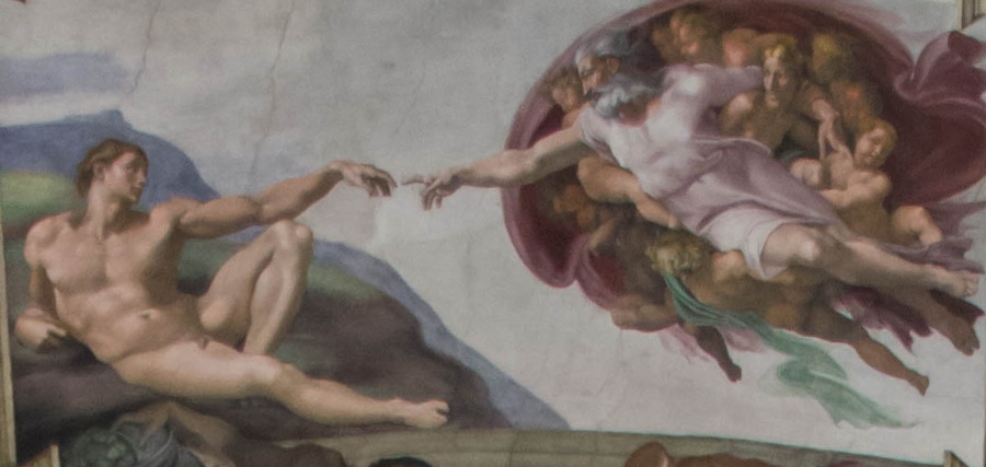
How future generations will study our culture:

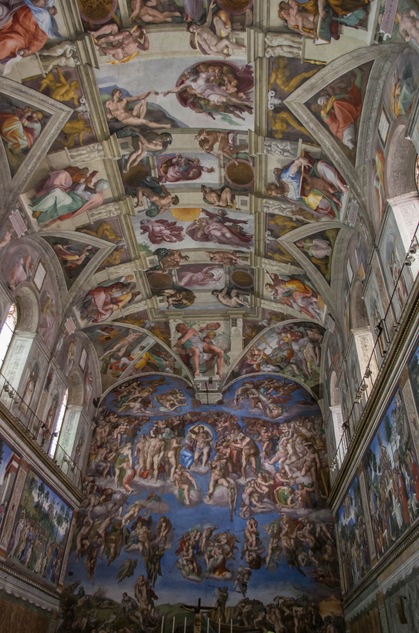
Our benevolent overlord:

Meanwhile, at Stanford:

---

What I learned

The most interesting thing I learned from this project is the process of feature extraction and matching. I’ve always wondered how to make a computer identify identical objects in different images. I think it’s cool that it can be implemented with really simple ideas, namely computing Euclidean distance between image patches (after appropriate normalization).