Project 6 Part A & B: Auto-Stitching Mosaics

Part 1: Image Rectification

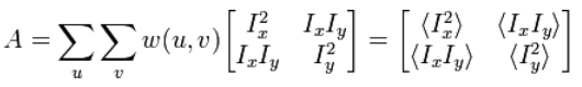
To rectify an image, I first compute the homography (projective transformation) between two sets of correspondences for the first and second image. For the first set of points, I used the object I am trying to rectify and for the second image, I chose a set of points representing the shape of that object from a head-on view. To calculate the homography transformation, we can solve a system of linear equations solving for a 3x3 matrix with the right most bottom value set to 1 using least squares estimate.

In the example below, I rectified a receipt on the table by warping the shape of the first image to the plane of the head-on shape I want.

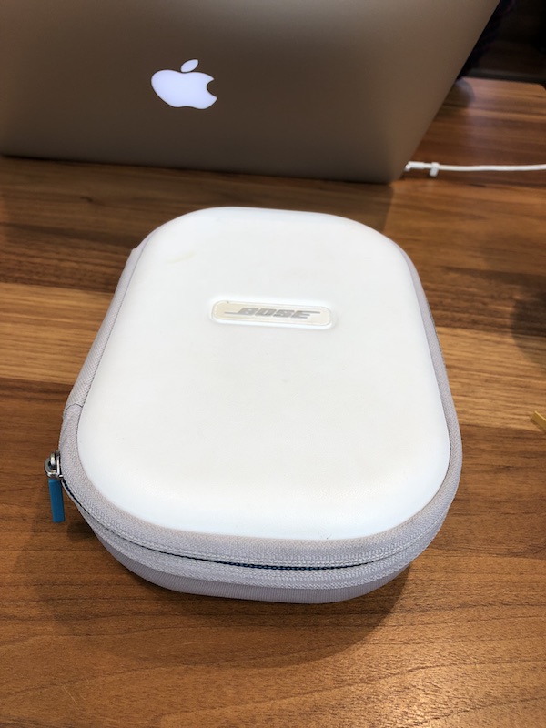
Here, I rectified this image of my Bose headphopnes case lying on the table to the rounded rectangular shape of the case.

Part 2: Blending Images Into a Mosaic

I took images from two different perspectives with the same center of projection. I want to blend my images into a panorama shot by warping all the images from different perspectives into the same image plane (center image). I do this with the similar method as the first part, except now I am warping corresponding points in the first perspective to the same points in the second. This will create a blended image with no seam, given that the exposure conditions and center of projection is the same. Here are my results:

Part 3: Feature Selection with ANMS

Harris Corner Detection

We use the Harris Corner Detection algorithm to detect the corners in our input images using the first-order derivative. A Harris corner (an interest point for all general candidates) is characterized by a large variation of S in all directions of the vector (x, y).

Here are the corners detected by Harris Corner Algorithm below. As you can see, there are a lot, so in the next part we want to limit the number of interest points as well as maintain equal spacing between points so they aren't concentrated in certain "stronger" parts of the image.

Selecting Features with Adaptive Non-Maximal Suppression Algorithm (ANMS)

ANMS is motivated by the fact that we want a fixed number of features per image, as well as an even spatial distribution of points. To perform ANMS, I sorted the images by their minimum suppresion radius, as defined in the MOPS paper. Then I chose the n strongest interest points to be my final feature set, with n being the number of features I wanted for my image (user-defined).

Part 4: Feature Matching

Feature Description

We define a feature descriptor as a description of a local image structure that will support reliable and efficient matching of features across images. To do this, we take a 40x40 patch around a pixel (the interest points chosen from ANMS) and downsample it by a factor of 5 to a 8x8 window. After sampling, we normalize the descriptor vector so that the mean is 0 and standard deviation is 1. Pictures below is a sample descriptor on one point in an image.

Nearest-Neighbor Algorithm (Russian Granny Algorithm)

We use Lowe's ingenius Nearest-Neighbor Algorithm described in this paper to calculate the candidates for matching pairs of points between two images. The concept is simple: based on the idea that correct matches between features pairs always have substantially lower error than incorrect matches.

Here are the features we have matched using the descriptors and Nearest-Neighbor algorithm described above on the descriptors of two images. As you can see, many of the matches are as expected on point. However, some are incorrectly matched (outliers). Which, is the topic of the next part of the project.

Part 5: Random Sample Conensus (RANSAC)

In this step, we randomly choose 4 sample points as corresponding points, and count number of points which agree with this prespective transormation and called it current_size. Finally, we return a homography matrix with the greatest number of inliers. In the final part, we use this homography matrix to calculate the transformation to stitch our images together.

Part 6: Auto-Stitched Mosaic Results

Manual Image Stitching

Auto Image Stitching

Manual Image Stitching

Auto Image Stitching

Other Mosaic

What I Learned

Although this project was indeed challenging, I definitely learned a lot about the topic of homographies and projective image manipulation that I wouldn't have from just watching the lectures. I think that after comparing the results of my manually chosen correspondences and the auto-selected ones, I realized that I am super bad at choosing correspondences, and the computer is much smarter AND faster at choosing correspondences than me. Finding correspondences for each image took me way longer than running Harris Corner Detection, ANMS, NN-Algorith, and RANSAC combined - which goes to show the power of computational photography.