CS 194-26: Image Manipulation and Computational Photography

Project 6: [Auto]Stitching Photo Mosaics

Tony Pan, CS194-26-adn

Part A: Image Warping and Mosaicing

Overview

This first part of the project focused on image warping and mosaicing. This involves manually defining point correspondences on one or more images, calculating the homographies between these points, and warping (and or blending) to achieve a result image.

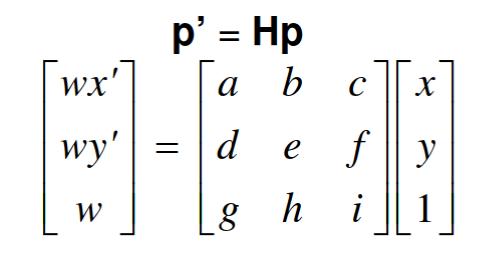
Part I: Recovering Homographies

This part involved calculating the homography H that allows us to map between different projections. In this case, using the equation below, we are able to create a series of equations that can be then solved using least-squares (provided more than 4 correspondences are given). The solution to the least-squares problem are the values a through h of the homography, with i being 1.

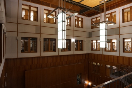
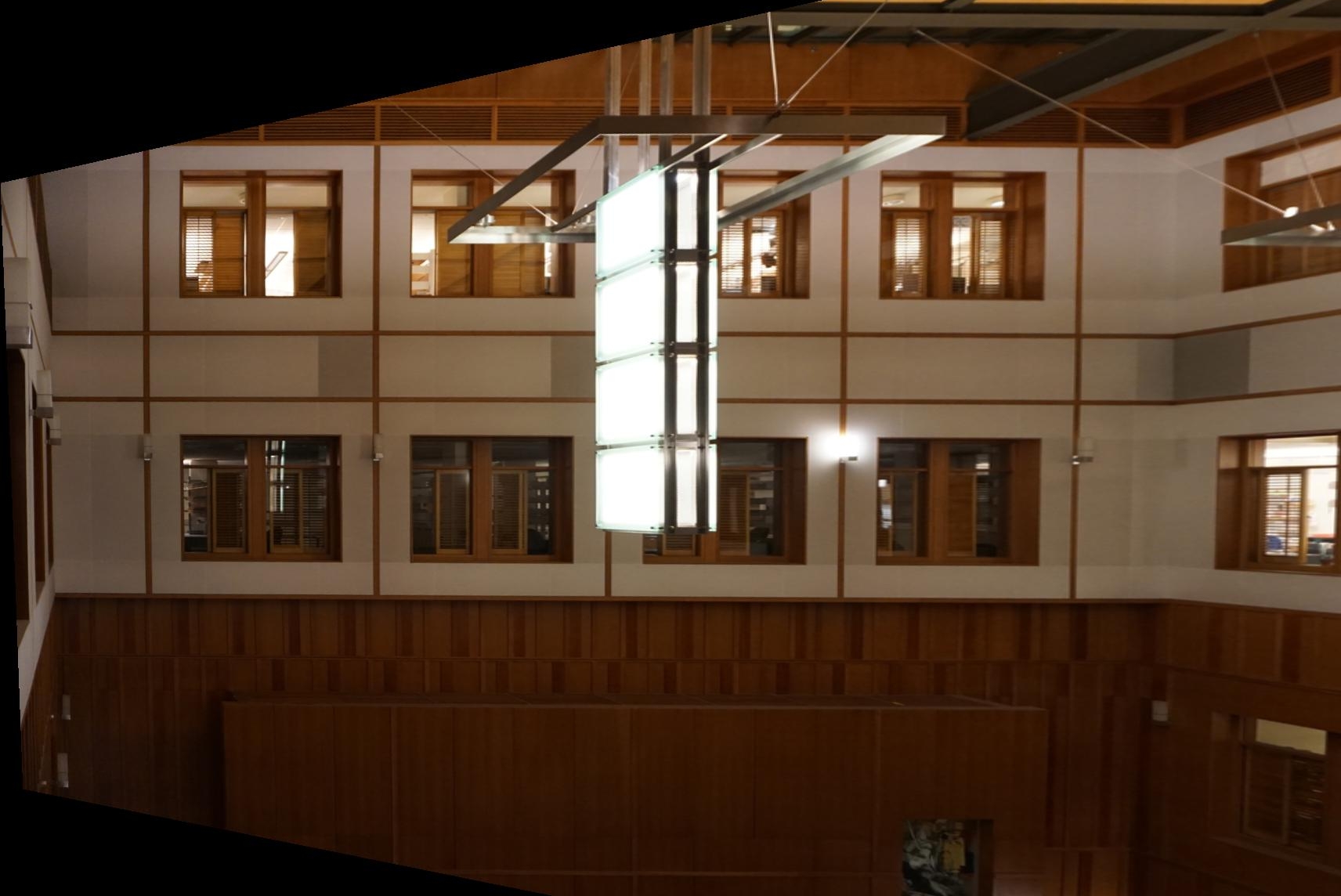
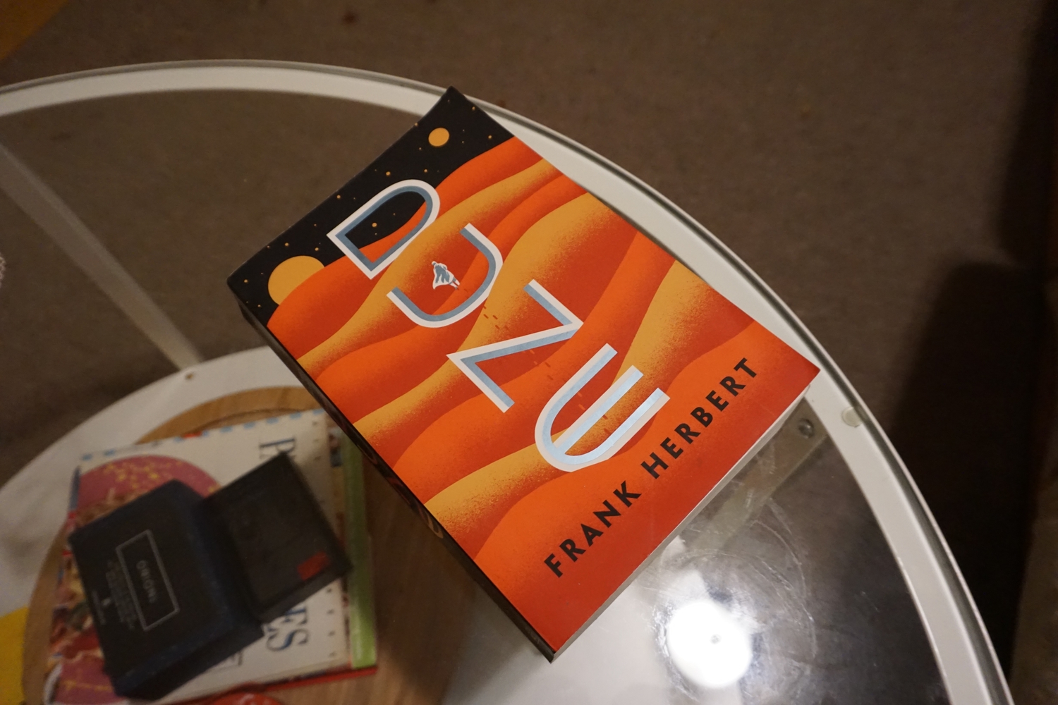
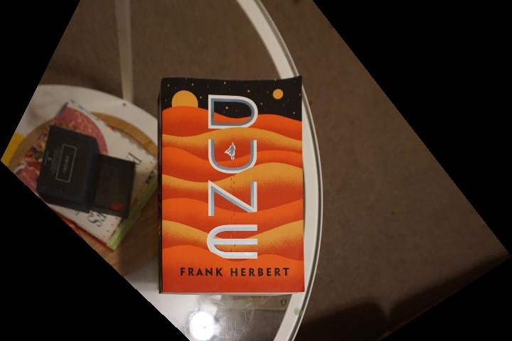
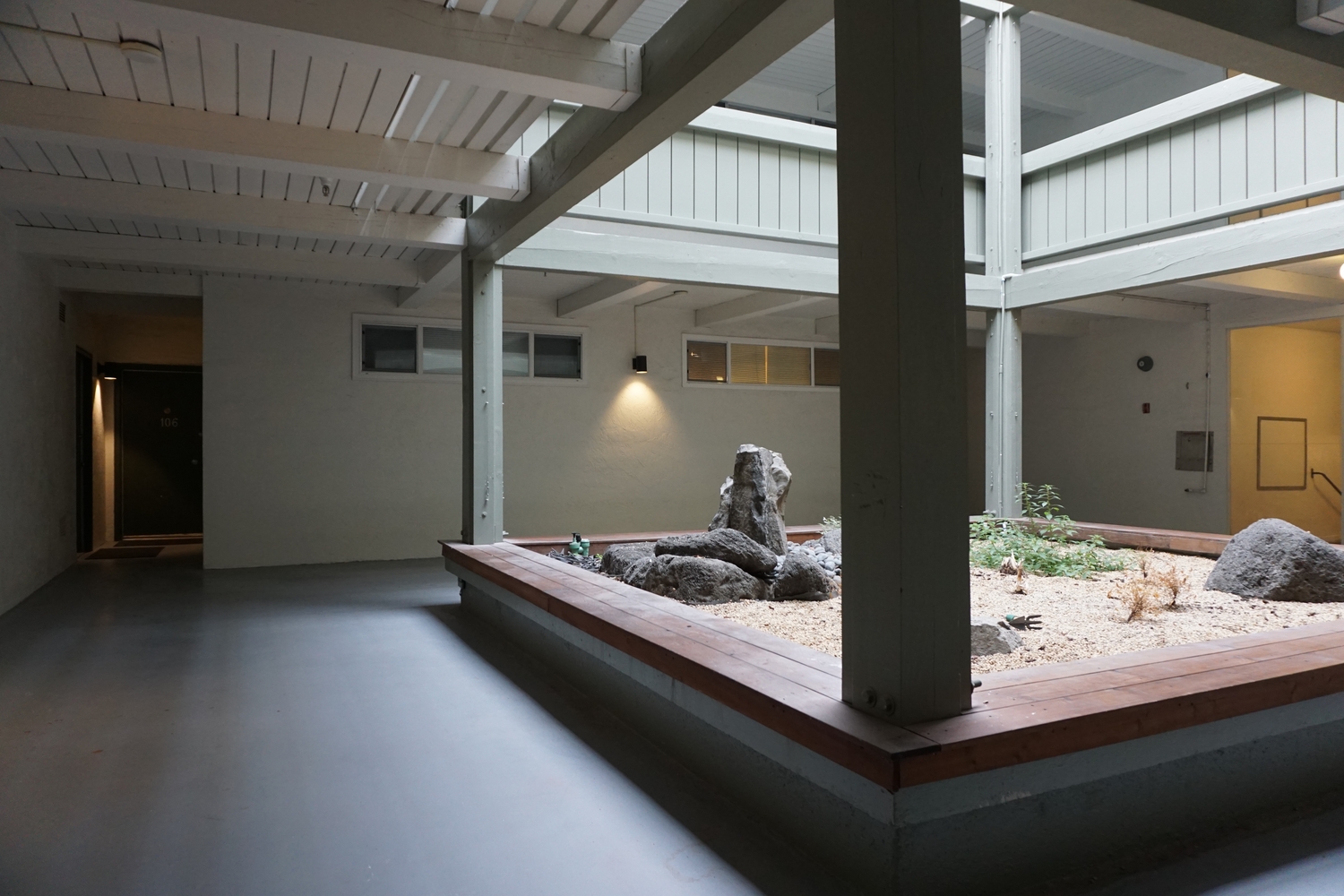
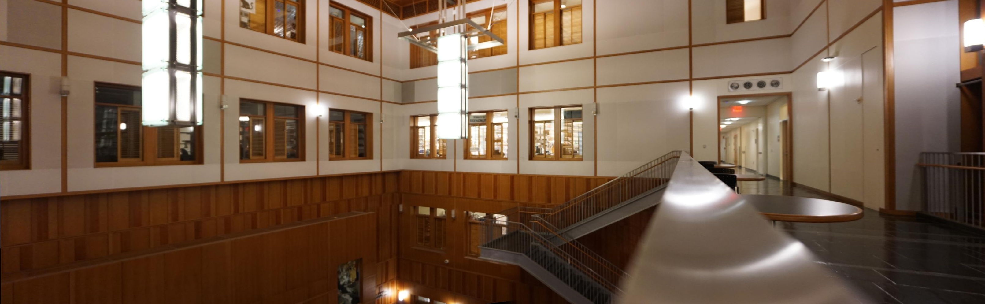
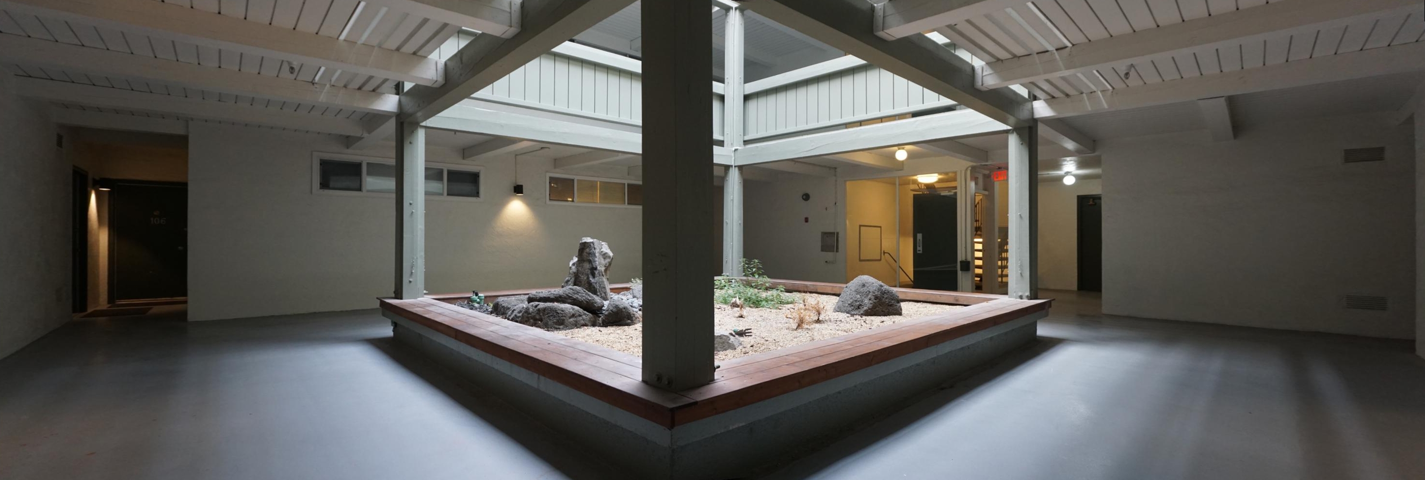
Part II: Image Warping & Rectification

Given the homography, it becomes relatively simple to warp or rectify an image. The process involves resampling the image using an inverse warp, such that values in the warped image are interpolated from the original. This process allows for some pretty interesting effects, such as warping an image such that a certain plane is front-parallel. The images on the left are before the warp is applied, and the right set of images shows the effects of rectification. As can be seen, both images have some planar surface that has been warped to be front-parallel.

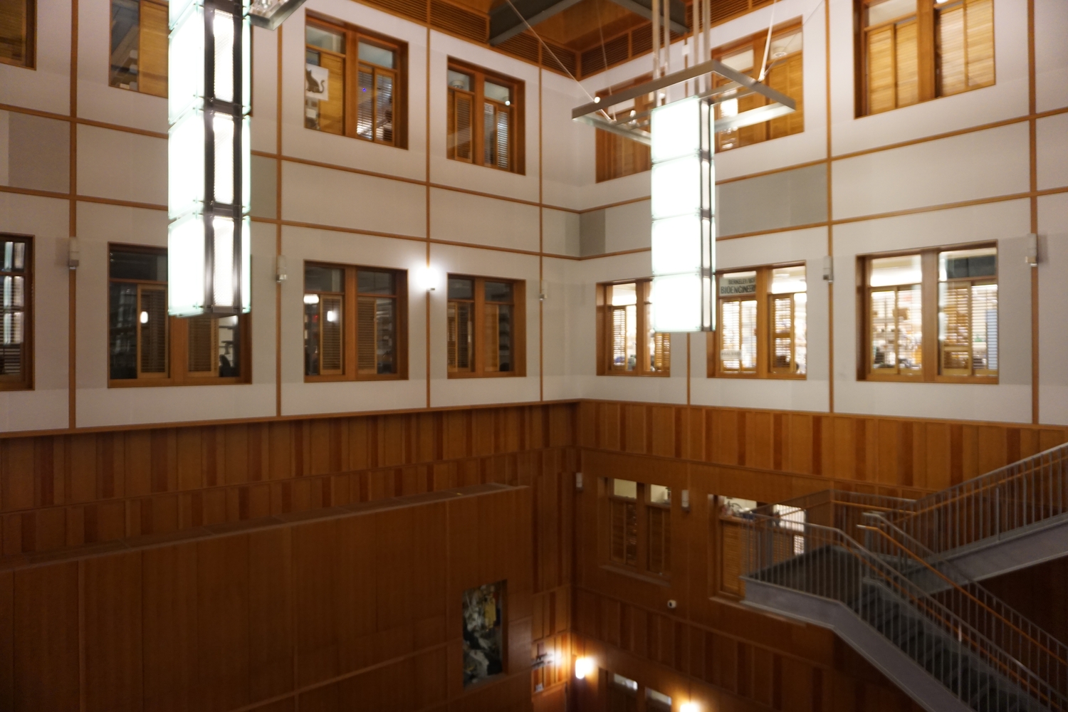
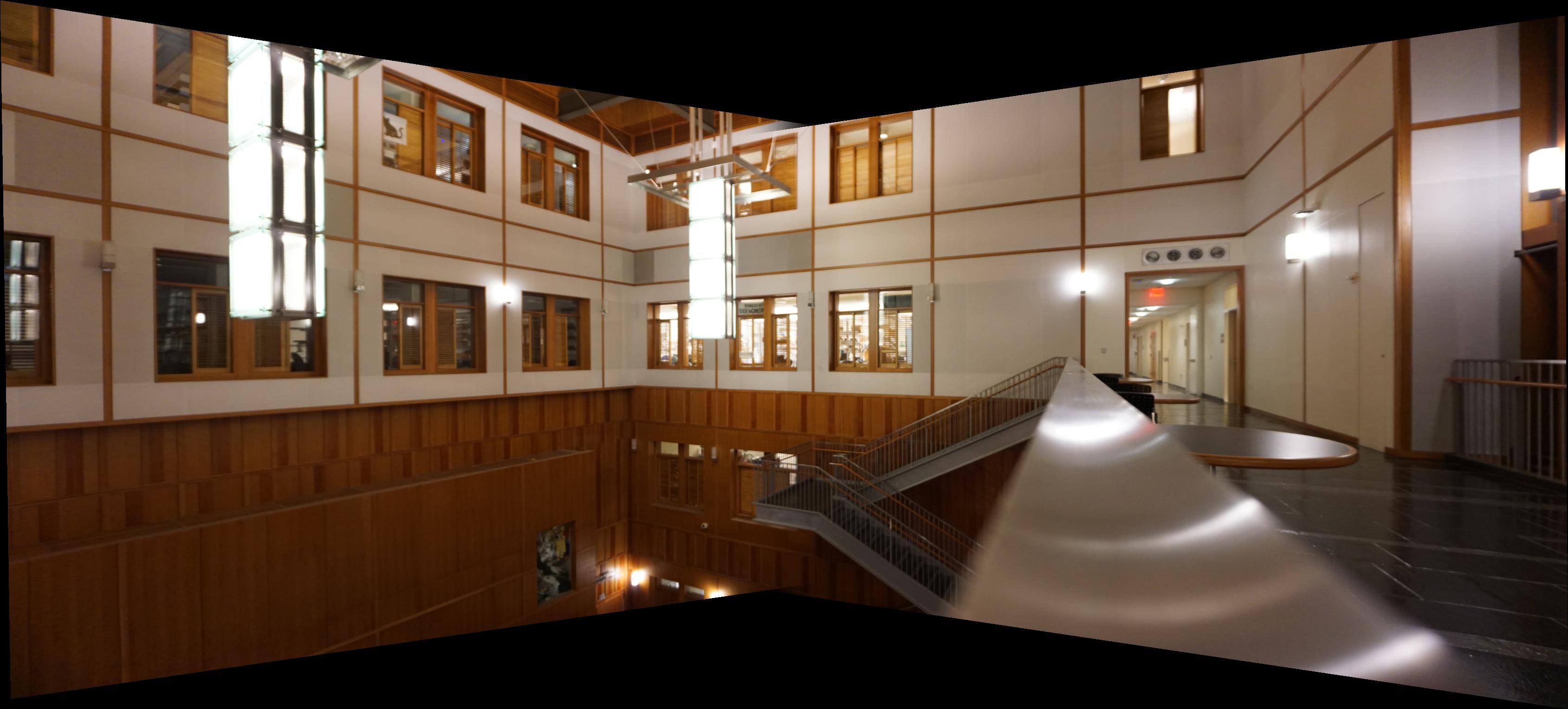
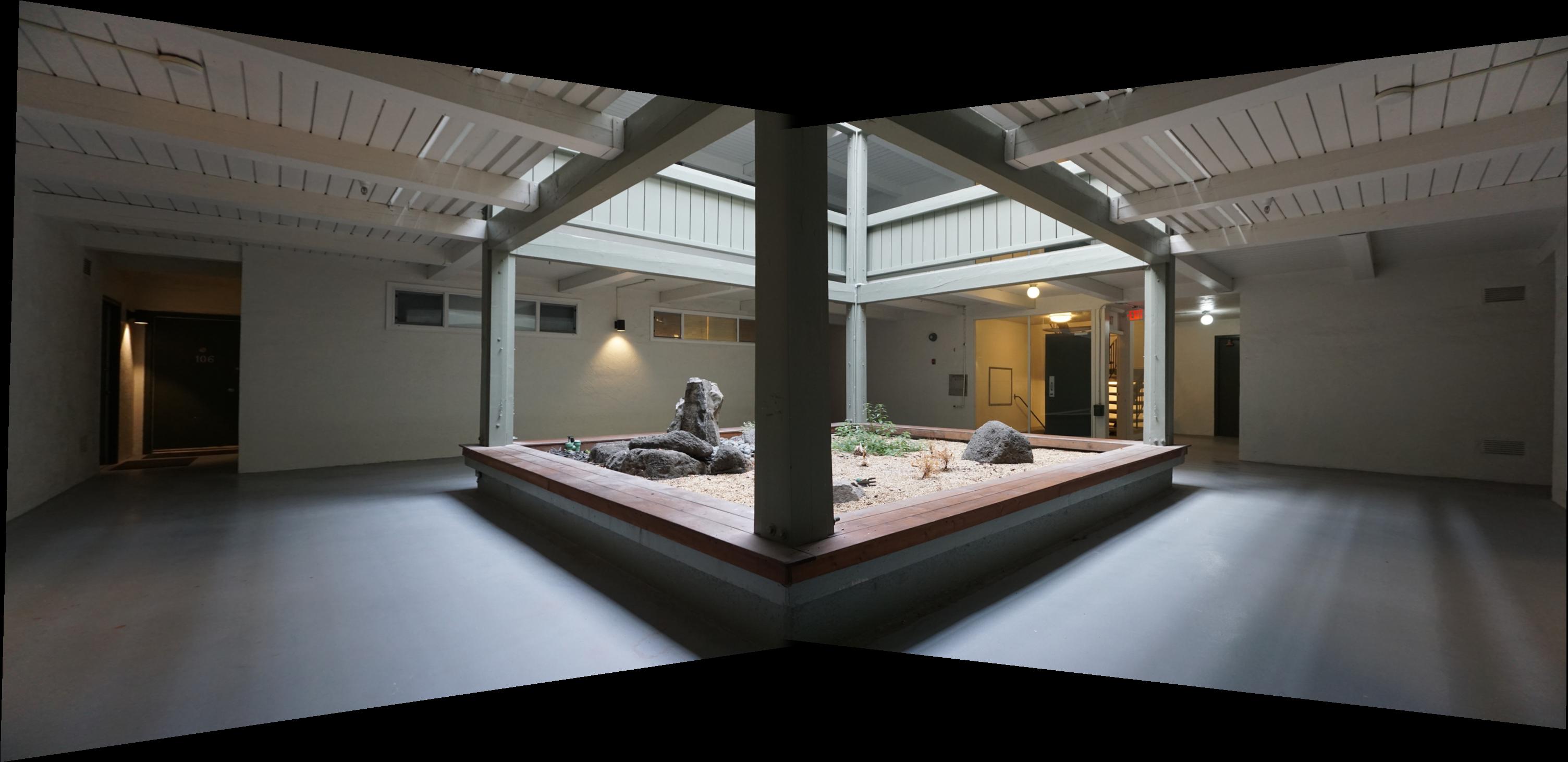
Part III: Image Mosaicing

Image mosaicing operates similarly to image warping, only in this case two images are warped to some central correspondence and joined. Defining matching correspondences was pretty hard using ginput, but I ended up getting some good results without having to pixel-match too hard.

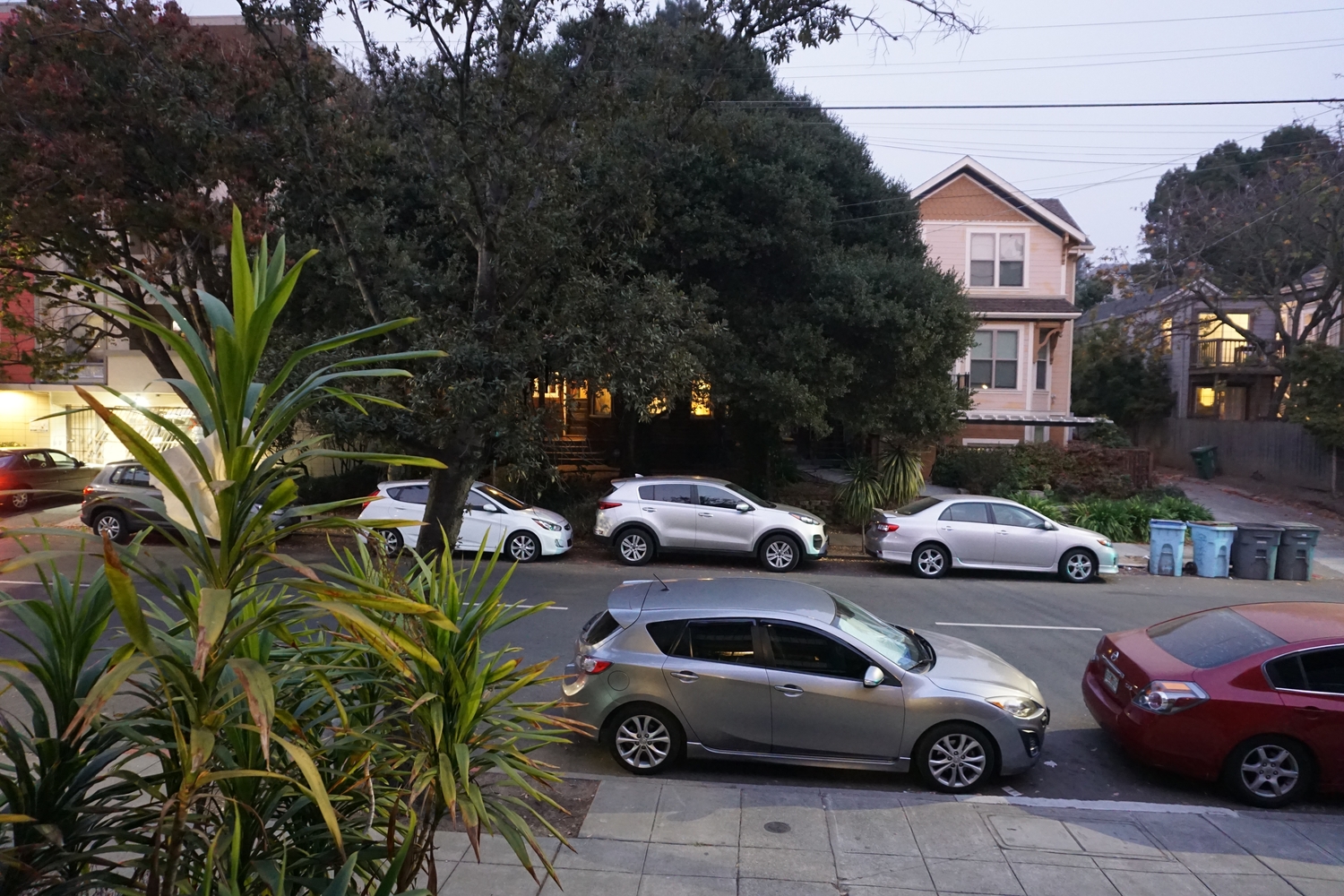
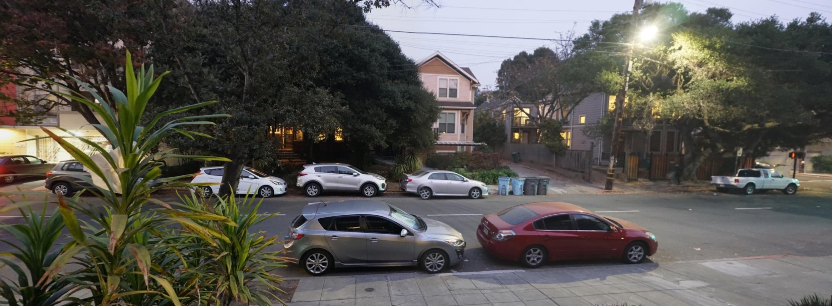
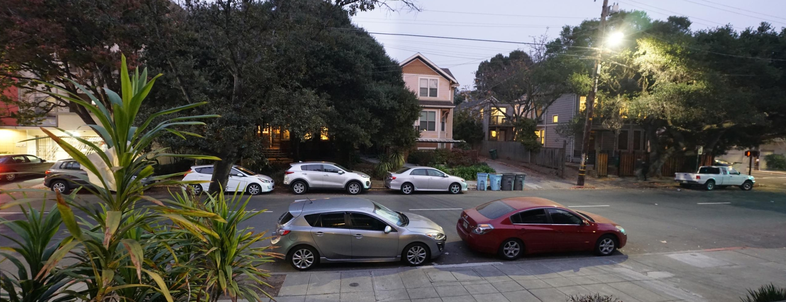
In the above mosaic, I had some trouble getting everything to match up, and there are still some artifacts visibile after laplacian blending. For instance the gray sedan in front of the house has some noticeable artifacts near its bumper area. Though it may be possible to achieve a better blend with better correspondences, this was the best result I got on that set of images. All in all, I think that this method of creating mosaics works quite well, so long as you are able to define correspondences that match each other closely.

Part B: Autostitching

Overview

Instead of manually defining correspondences as in the last project, this next part uses Harris corner detection, Adaptive Non-Maximal Suppression, feature matching, and RANSAC to automatically come up with a set of viable correspondences. This results in a faster and pain-free process of mosaicing, with absolutely no pixel peeping required.

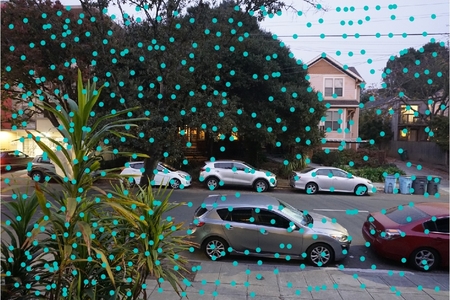
Part I: Detecting Corner Features

Corners are relatively easy to pinpoint, and as such are a great way to define 'points of interest'. Harris corner detection is used to find corners, by examinng differences in pixel intensity within a given neighborhood. The code needed to run Harris corner detection was (thankfully) already provided. Running corner detection yields several thousand points, many of which will eventually be discarded through ANMS and RANSAC. Some examples of corner detection outputs are shown below.

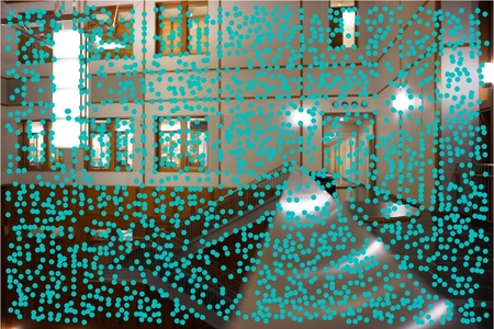
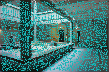
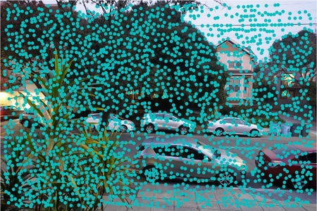
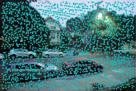
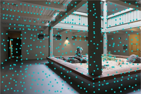
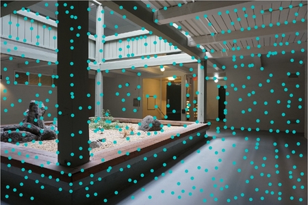
Part II: Adaptive Non-Maximal Suppression

Harris corner detection yields far too many points, so some means of suppressing the number of interest points in an image is needed. Adaptive Non- Maximal suppression allows us to restrict the number of interest points, while making sure they are well distributed throughout the image. ANMS essentially chooses the 'strongest' corner within a certain radius r. The n points with the greatest r are retained, and the rest of the points are discarded. The images below show the effects of ANMS, with n = 250, 500, 500 for each row respectively. In practice however, I chose to use n > 1000, as it ended up yielding a greater number of correspondences later and generally resulted in a better mosaic. This was largely dependent on the images I was blending, as some would work just fine with 250 or 500 interest points, while others needed far more.

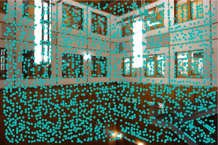
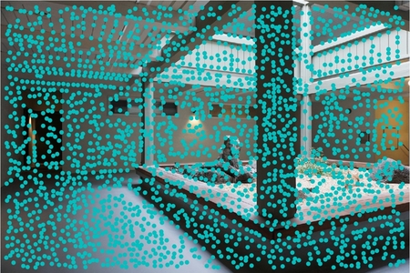
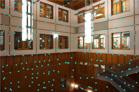
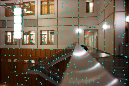
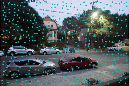
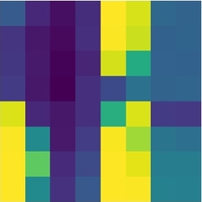
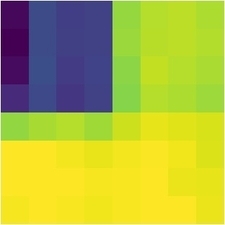
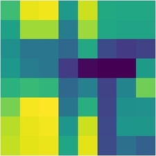
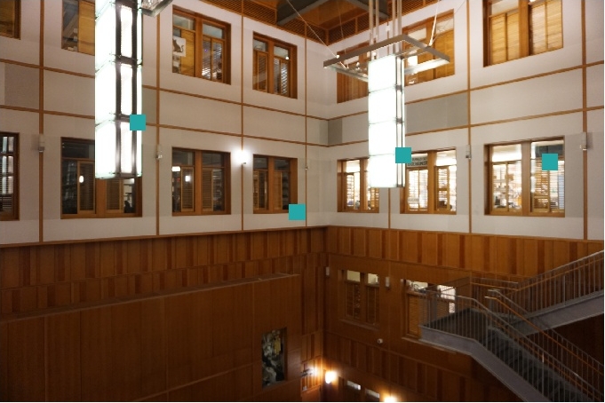
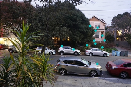
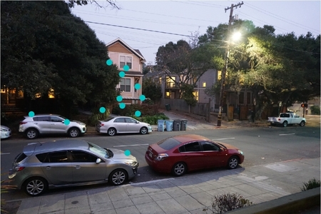
Part III: Feature Extraction And Matching

Having sufficiently suppressed the interest points, we must now extract actual features from the images, to use in feature matching. To do so, we take a 41 x 41 pixel patch around a given point of interest. This patch is then downsampled to 8 x 8 pixels in order to make features less sensitive to noise and small shifts. Features are then bias/gain-normalized, such that their mean is 0 and variance is 1. Some example features taken from an image are shown below, with each teal square on the bottom image corresponding to its respective feature.

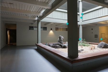
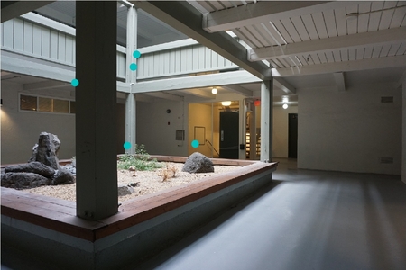
Part IV: RANSAC

Because there might be incorrect points left over from feature matching, we use 4 point RANSAC(RANdom SAmple Consensus) to find a set of correct correspondences from which a homography can be calculated. The process is pretty straightforward, and involved repeatedly taking 4 sets of points randomly and computing a homography on them. This homography is applied to the complete set of points, with each warped point being compared to its corresponding matching point. If a warped point is sufficiently close to its matching point, then it is added to an inlier set. This process is repeated many times (I ran 1000 iterations), and the largest inlier set is used to compute a robust homography used in mosaicing. As can be seen below, RANSAC is very good at finding matching features.

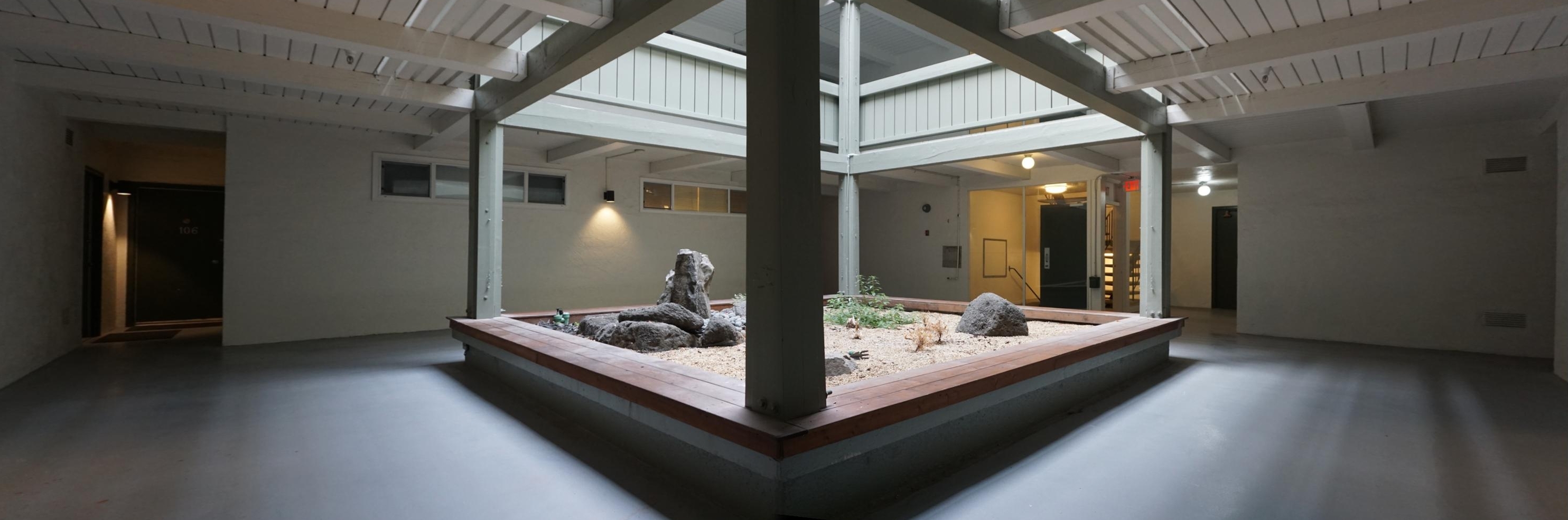
Part V: Autostitching Results

The results of the autostitching results, as well as the manual-correspondence mosaics are shown below. In each pair of images, the top image is the mosaic generated from manually entering correspondences, and the bottom image is from autostitching.

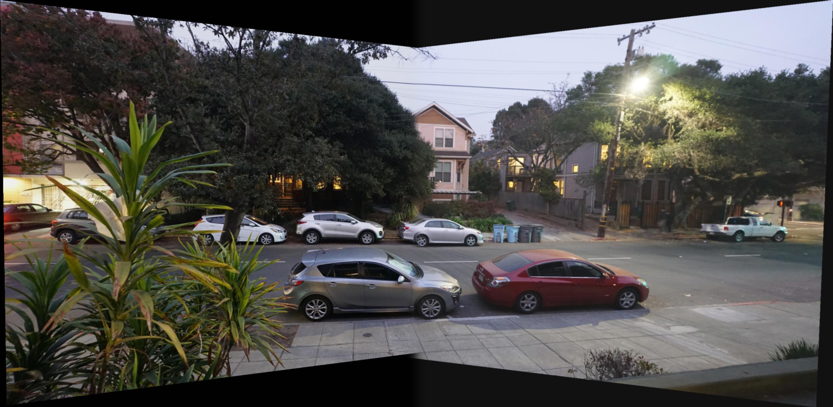
For the most part, autostitching yields a result that is at least as good as the mosaics from the previous part of the project. The first two pairs of mosaics are virtually indistinguishable from one another in overall quality. There is a visible improvement in quality in the third autostiched mosaic, where visual artifacts previously visible on the gray sedan and sidewalk have been resolved. It was a painstaking process to define correspondences manually, and I often had to repeat the process many times to get a good mosaic. Autostiching makes the process many times easier by removing the imprecision of human-entered correspondences, and instead using automatic feature matching. The only major issue I noticed with autostitching was that I would sometimes have to tweak certain values to achieve an ideal result, but it was overall a far superior method of mosaicing than manually recording correspondences.

Part VI: What I Learned

It was very cool to see how an automated process could find and match features in a set of images, to create a mosaic of better quality than a person could. There were some very interesting algorithms used, like RANSAC and ANMS, that were pretty ingenious in helping yield a better result. Overall, it's a pretty magical process to watch unfold, and I think it's pretty amazing how good the results consistently are.