The fundamental basis of this part of the project is to get familiar with image warping how how it can be used
to stitch together a familiar concept: panoramas. In order to do so we will be using homographies to warp our images into
the correct perspective and then stich them together.
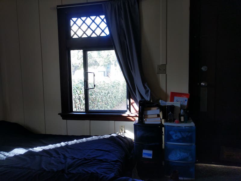
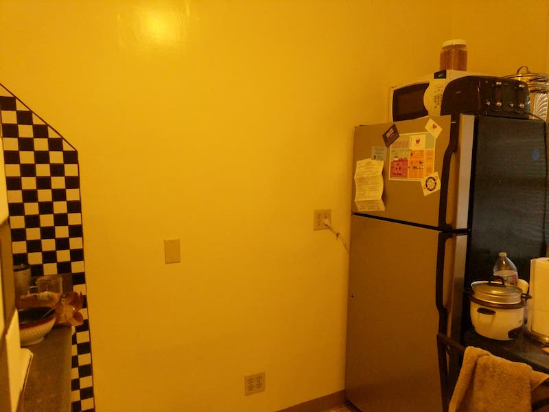
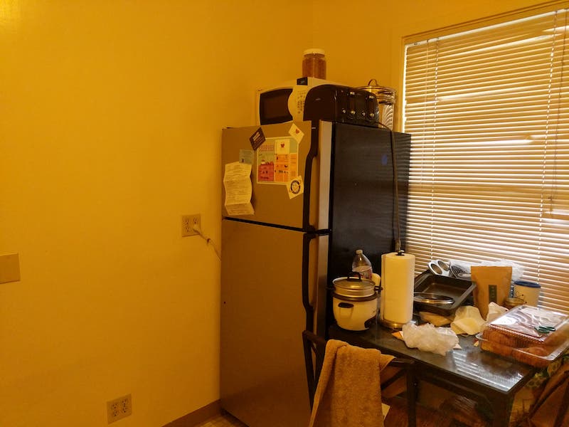
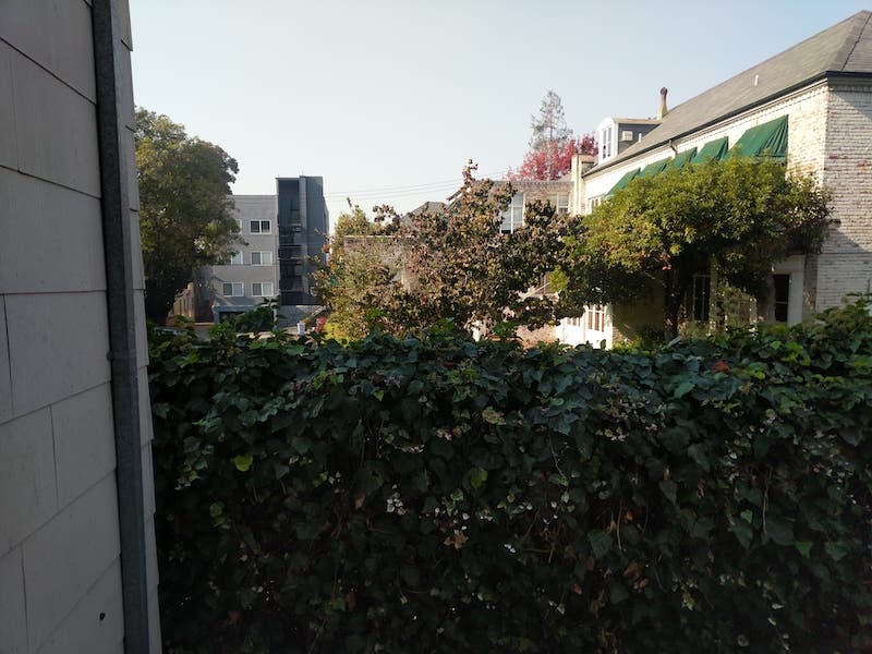
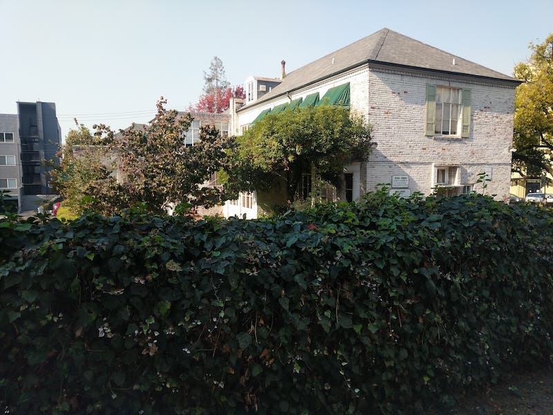
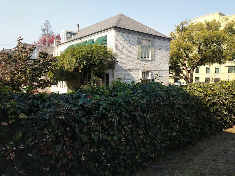
Here are the input images used:
Similar to face warping we must find a matrix that transforms one set of points to another.
This way, we can define correspondence points manually on our photos to stich them together as well
as adjust the perspective of the photos to form a "seamless" panorama. This can be solved be setting up
a system of linear equations solving for a 3x3 matrix with the right most bottom value set to 1.
With our homography 3x3 matrix, we can now transform each pixel in the image. In this case, we follow the same
method of inverse warping that we used in face warping. This way we can use interp2d to fill in any of the stretched out pixels
since the perspective of the image is changing.
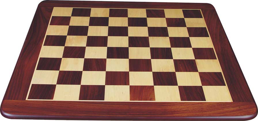
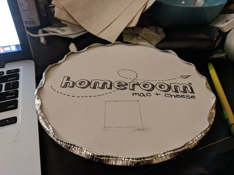
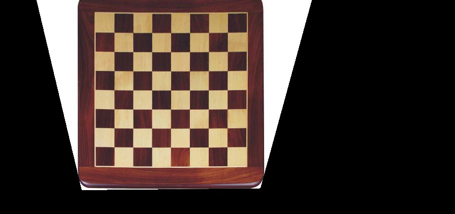
As a first step to show our warping abilities we can rectify images at an angle. In this case we start with an easy example,
as chessboard which clearly should be a square. We also just assume a square when setting the points for the image and the user specifies
the pixel height of the intended square.
This part of the project was definitely incredibly interesting and super relevant to stuff
we do on a somewhat daily basis. Although what we did was very basic compared to modern panoramic systems
it was still neat to come out with results that didn't look too bad. After the face morphing and this project,
I'm really starting to see how powerful transformation matrices can be and the many applications of them. On top,
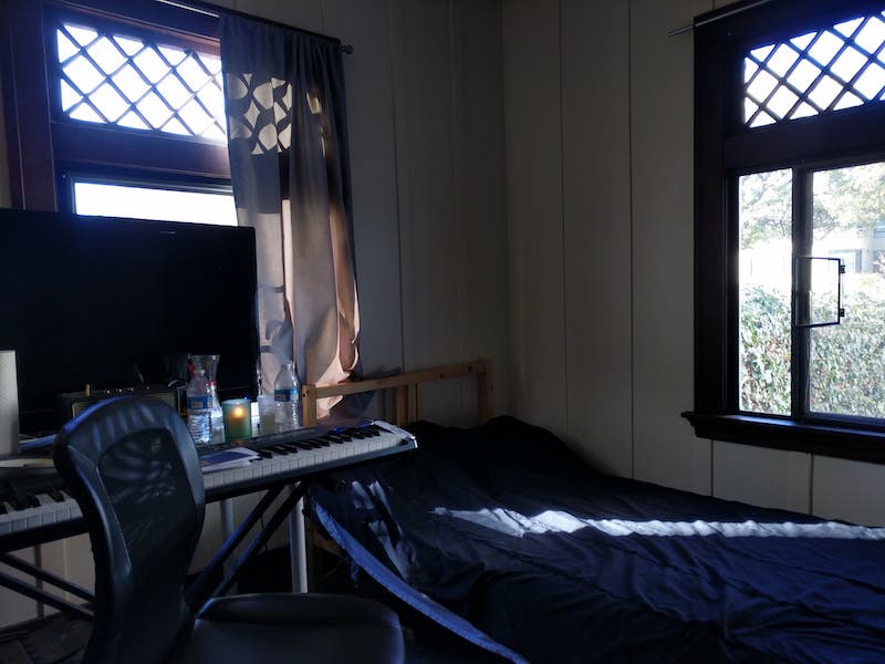
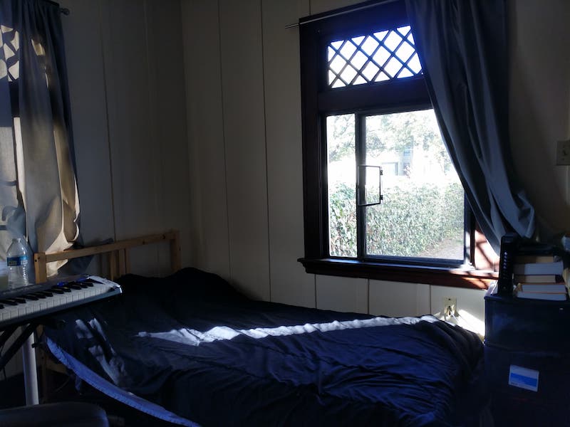
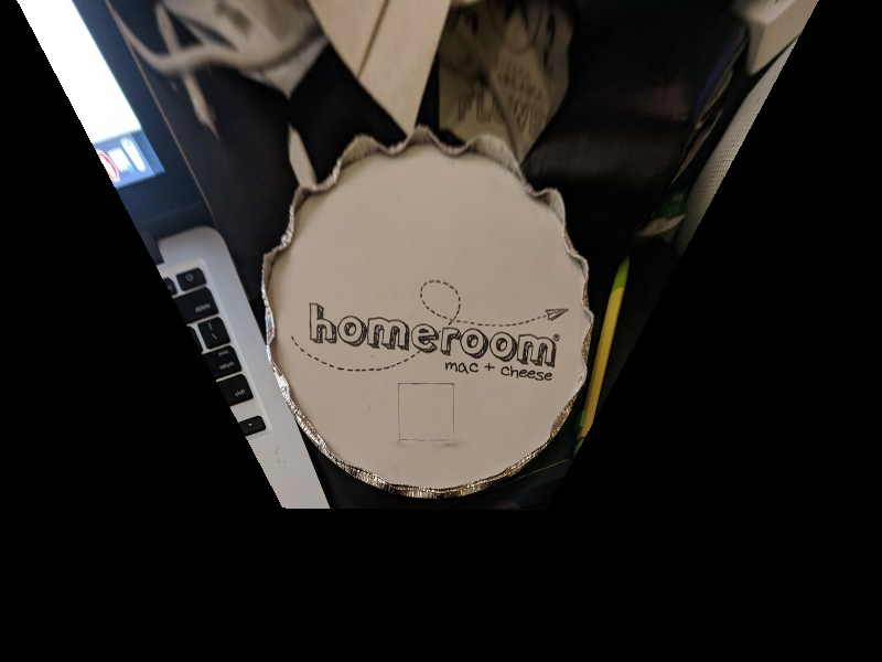
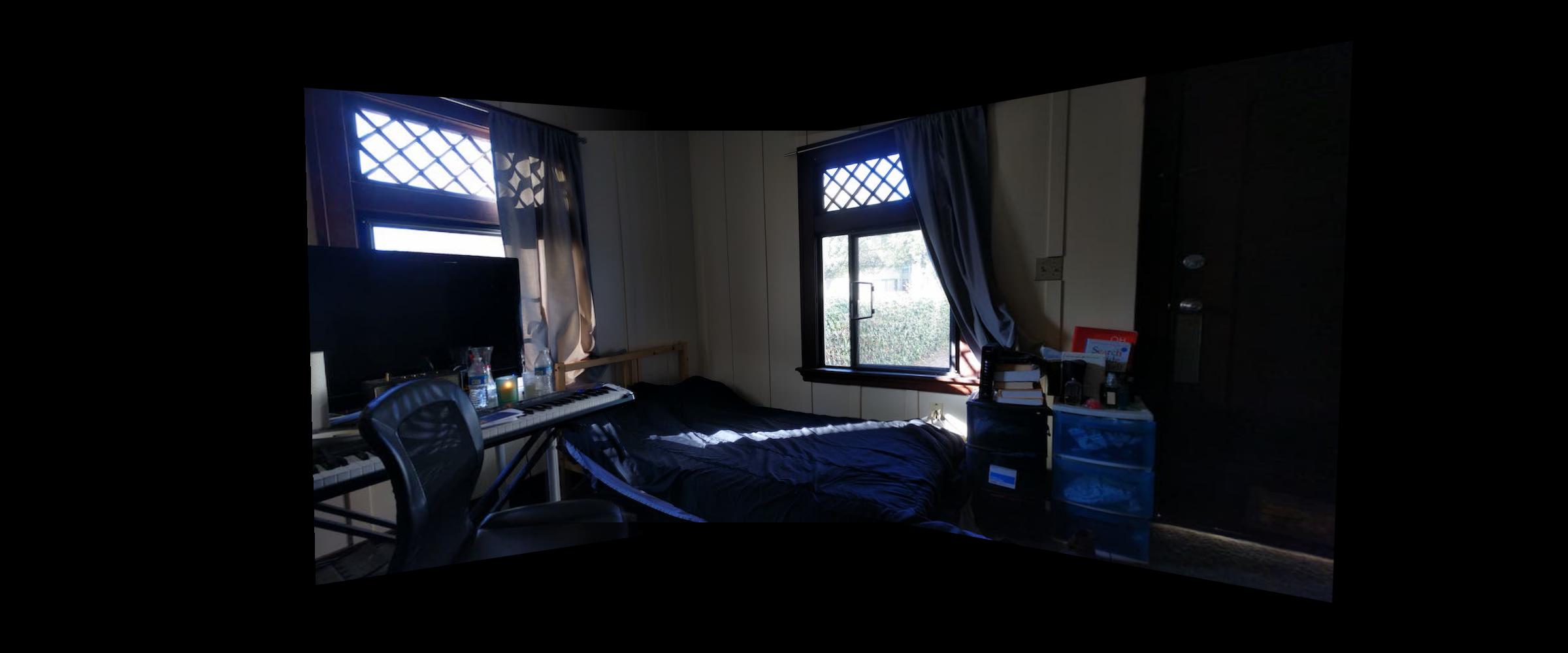
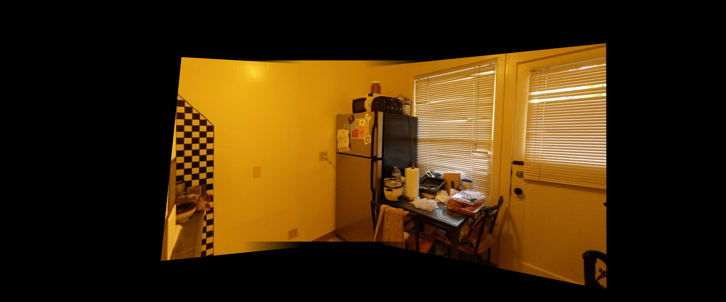
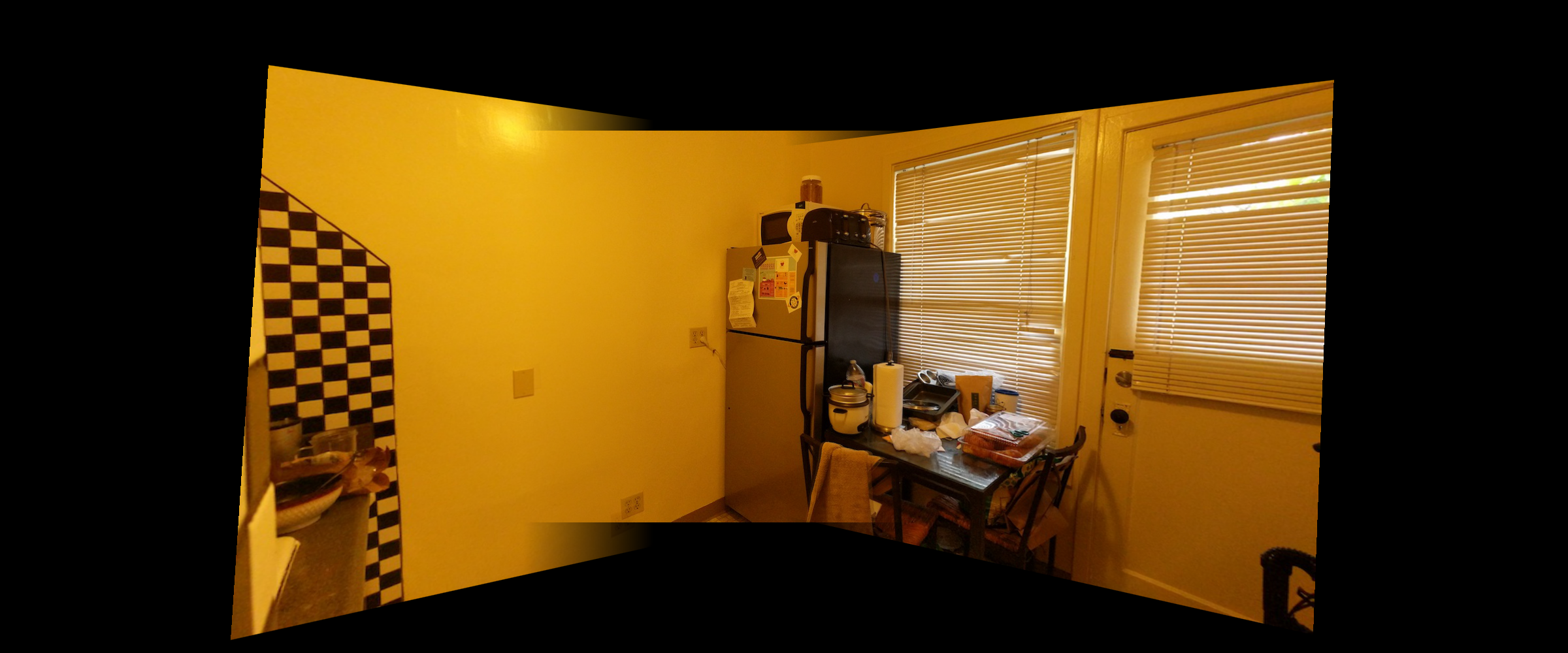
it's great to go back and use the blending techniques from early on in the semester. Here are a couple examples of no blending
and then blending. Notice the color changes at the cabinets and cut at the keyboard.

Part 2: Automatic Panoramas
The fundamental basis of this part of the project is to use the techniques from part 1 to
create automatic panoramas instead of specifying correspondence points. Essentially we start with
finding corners with Harris corner detection, limiting those corners to be spread out, and
finding matching points by comparing patches at each point. Then out of those matching points,
we use RANSAC to choose the best combination of points to find the best homography.
Harris Interest Point Detector
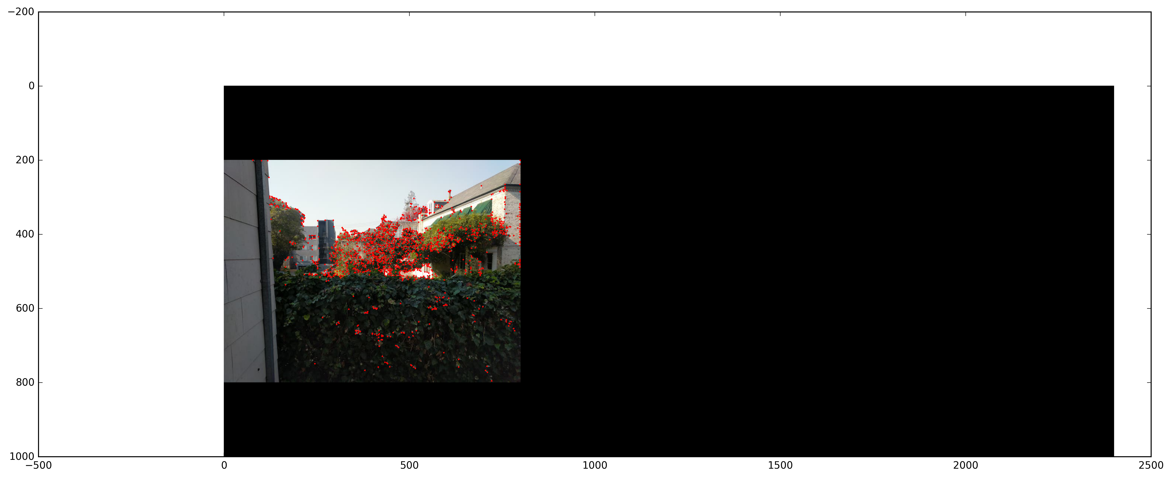
Using given starter code, we find Harris interest points by finding their corner response. We exclude
points near the border since we eventually want to use 40x40 patches. Here's an example of Harris corners
for our images. We also limit harris points since the next step is incredibly computationally expensive.
Adaptive Non-Maximal Suppression
There are a lot of harris points. In order to fix this,
we want to spread the points out as well as retaining incredibly strong harris corners. In
order to do so, we try to find the minimum supression radius ri for all Harris points xi
using the following formula.
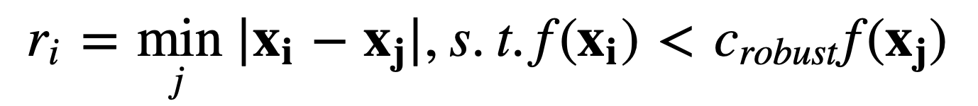
Note the c_robust variable which ensures that we only choose strong corners and f represents
the function that returns a points corner response. Simply put, we keep the xi with the 500 largest
ri where ri is the minimum radius where a nearby corner has a significantly larger corner response.
Here's an example of spreading out the points. You can see the points are much more spread out.

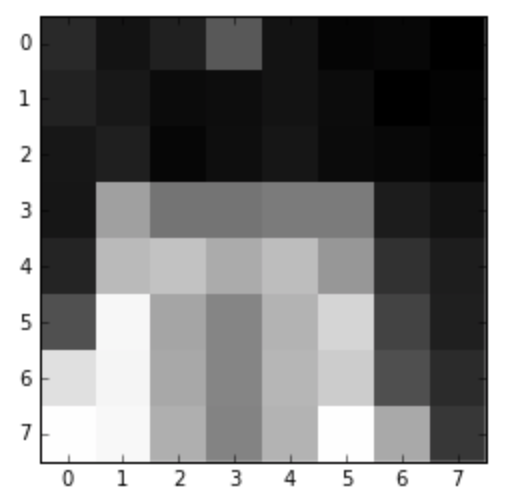
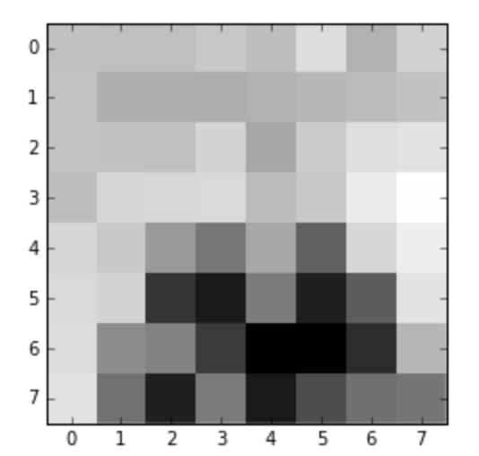
We can find corresponding points by using feature descriptors, which are essentially patches
surrounding each point which are 40x40. We take this patch, convolve with a gaussian and downsize it
to 8x8 and bias/gain normalize so we only care about the important low frequences and not small discrepancies
between shifts in color and artifacts. Here are a few examples.
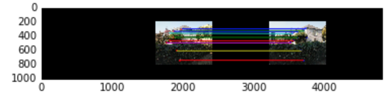
Now that we've found features, we can now match the descriptors by simply finding the SSD
between the descriptors. We only care about good matches though that are unique so we rank the
best 2 matches and find the ratio between the SSD of NN(nearest neighbor) 1 and NN 2. Thus if the
distance of the first neighbor and our patch is significantly smaller than the second, then
our features are likely good matches. Here's what we get with a ratio threshold of 0.2 for
the matches.
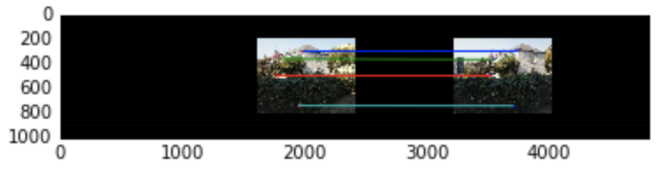
Now there are too many matches and some are inaccurate so how do we limit to the best matches? We can
use RANSAC to find the best 4 point matches. The algorithm simply finds a random 4 points calculates the corresponding
homography and warps each of the matched points and sees if the warped point is within 3 pixels of the actual second matched point.
We find the best random 4 point match with the most points within the pixel threshold and use that to transform
the whole image. Here's what RANSAC chooses for the photo above.
Manual
Auto
Manual
Auto
Manual
Auto
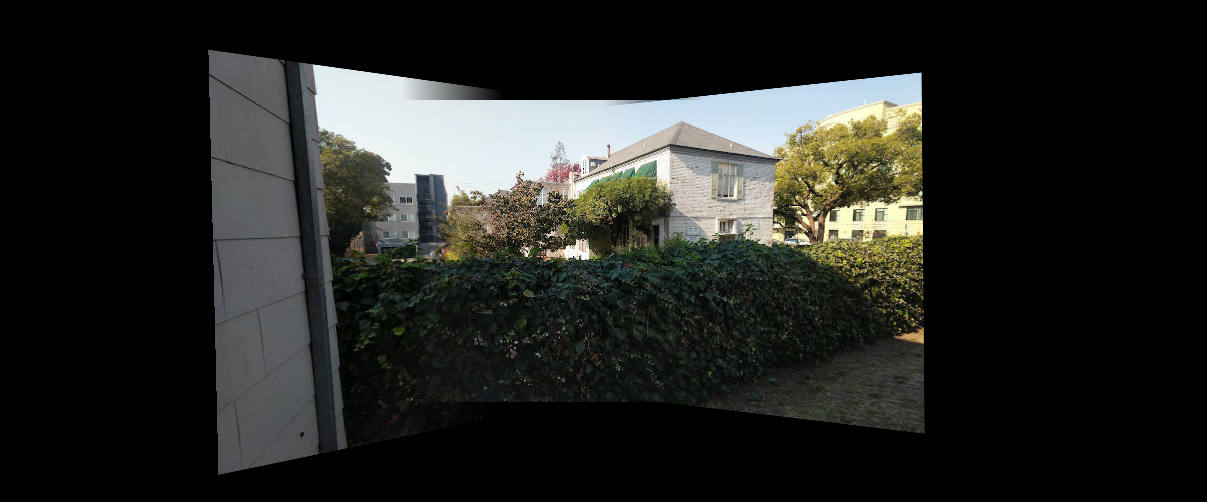
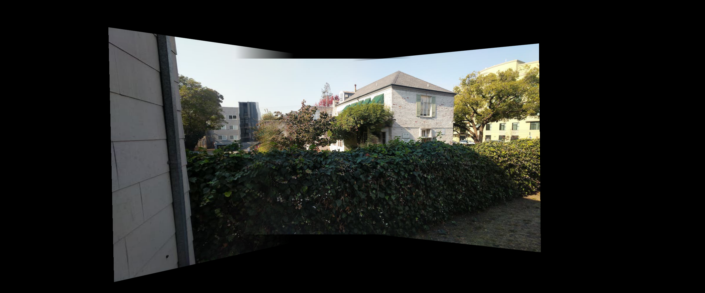
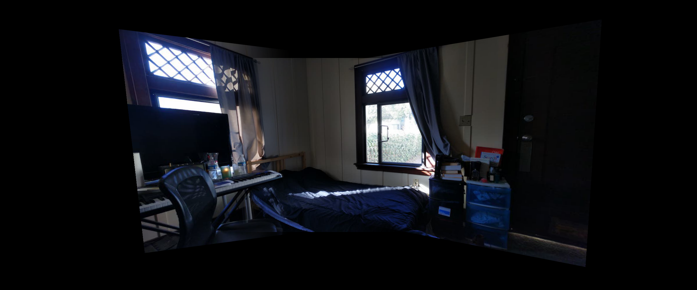
After finishing this part we can see some interesting results. The automatic alignment
helped some parts, like in the first image where the leaves are more aligned, but doesnt help
for other things like the buildings in the first image. It was really interesting to learn how to
automatically align but to be honest the time to finish all the automatic processes took longer than
manual points, which is unfortunate. But it's definitely cool!