CS194-26: Image Manipulation and Computational Photography
Programming Project #6 Part 1: Image Warping and Mosaicing
Allyson Koo
Project Overview
This assignment involved creating panoramas/image mosaics out of a series of pictures taken of a scene from the same center of projection. In order to do this, it involved calculating homography matrices between different images in order to be able to warp one image to the same plane as the other, and then stitch them together into a panorama.
Implementation
Part 1: Shooting and Digitizing Pictures
This portion of the project involved taking two or more pictures that had some overlap and were projective transforms of each other. This can be accomplished by taking two pictures of different portions of a scene from different points of view. Example input images are shown with the mosaics produced below.
Part 2/3: Recover Homographies and Image Warping
The purpose of this portion of the project was to define correspondence points between two images by hand, and then calculate the homography matrix that represents the transformation between the two sets of points. Once the homography matrix is calculated, you can use this to transform all the points in one image to the same perspective as the other image. Once this is accomplished, you can now blend the two images together seamlessly to create a panorama style image. Examples shown below.
Part 4: Image rectification
The purpose of this portion of the project was to take images and make them frontal-parallel, using the homography and image warping techniques as described earlier. Since we are warping a single image in this case, for my second set of correspondence points I defined them by hand to be rectangles/squares in accordance with the pictures. Examples shown below.
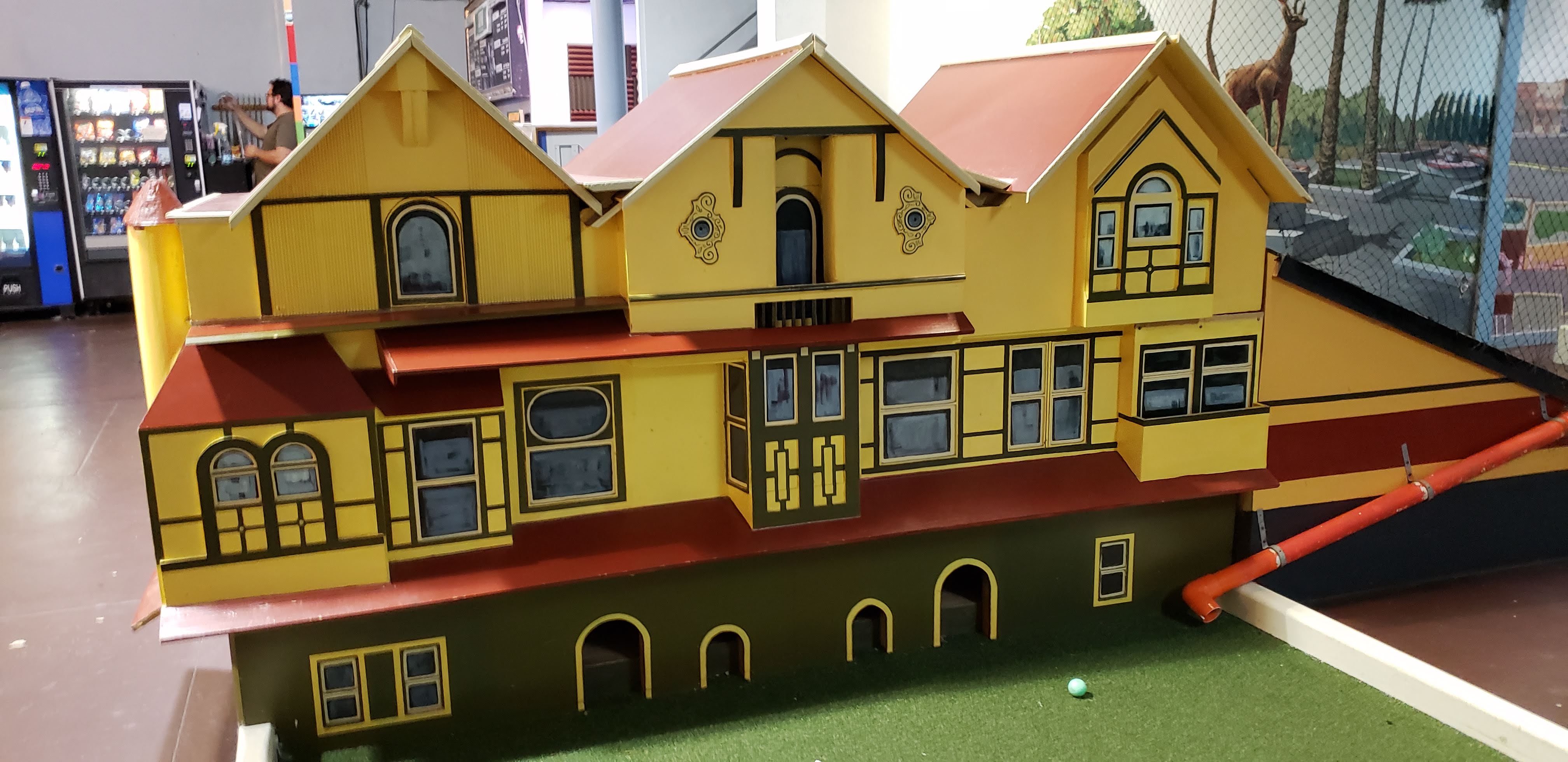 Original image: wooden house on a mini golf course
 Rectified image
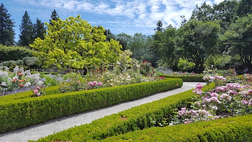 Original image: garden
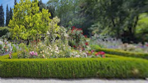 Rectified image
For the garden image, since the right side of the image had fewer pixels representing the necessary data, the right half of the rectified image is significantly blurrier than the left half as a result.
Part 5: Blending the Images into Mosaics
The purpose of this portion of the project was to combine the previous parts by blending the warped images together into a single panorama image. This was accomplished by warping one image into the perspective of another, and then copying the pixels over onto a final image that was four times the size of the original images. For the overlap region, different techniques were used to try to minimize the appearance of a seam between the two images.
Original input images:
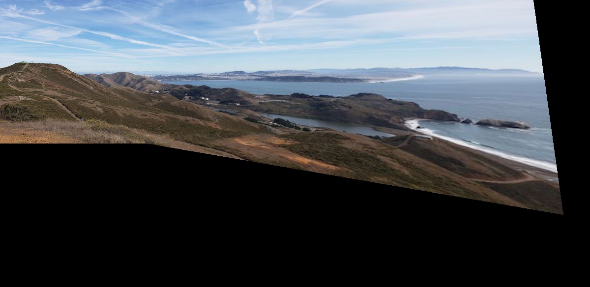
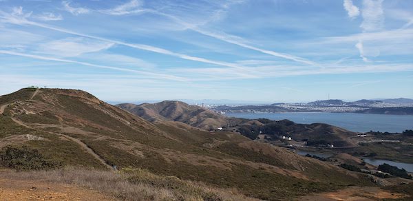 Original image: left half of view from Mt. Tam.
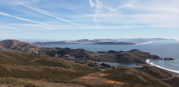 Original image: right half of view from Mt. Tam.
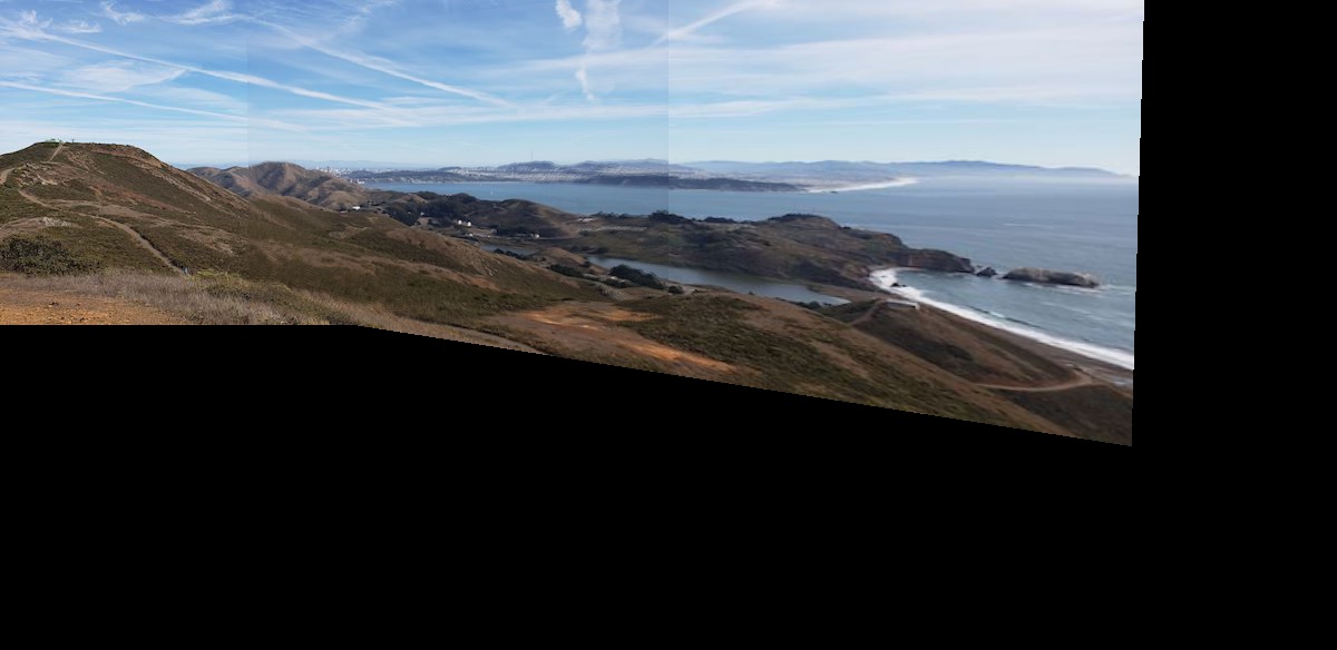 Combined images, using linear blending
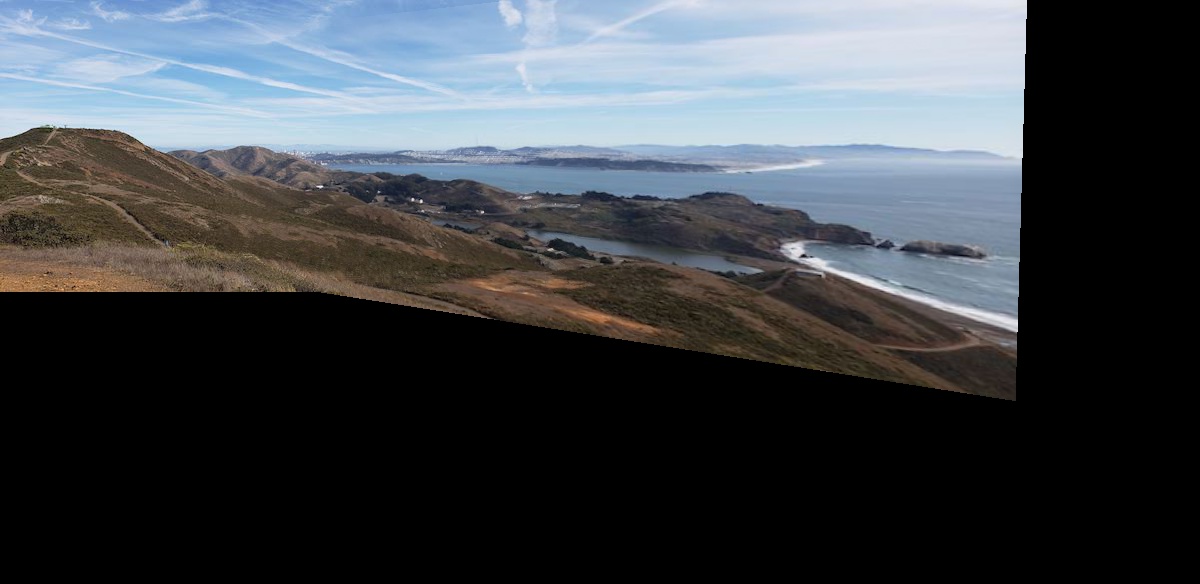 Combined images, using np.maximum for selecting pixels in overlap region
Example morphings of original faces into the average shape.
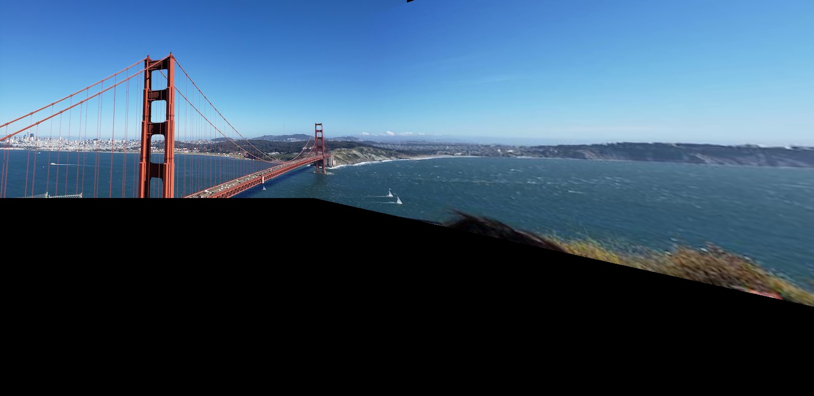
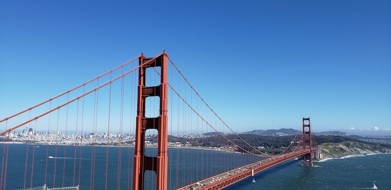 Original image: left half of view of Golden Gate Bridge
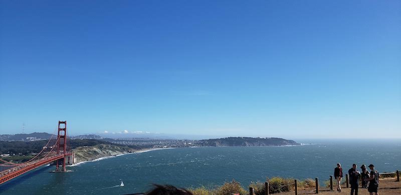 Original image: right half of view of Golden Gate Bridge
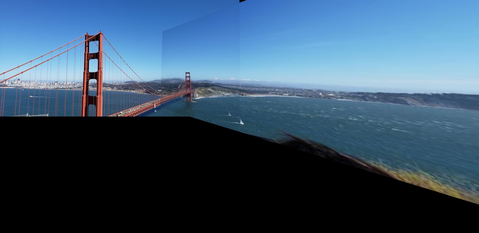 Combined image, using linear blending
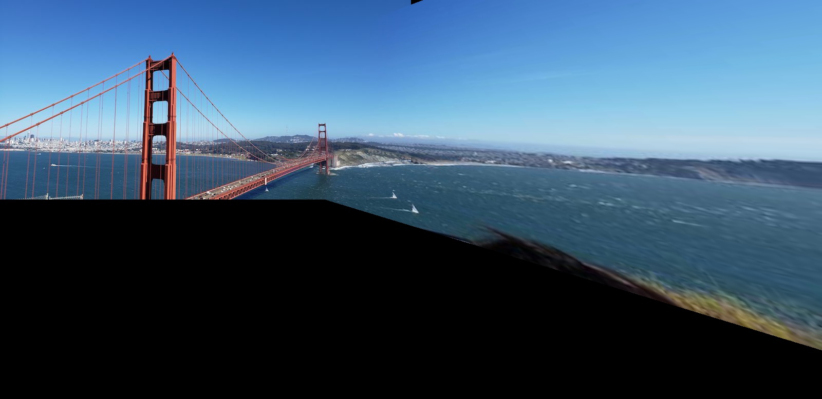 Combined image, using np.maximum for selecting points in overlap region.
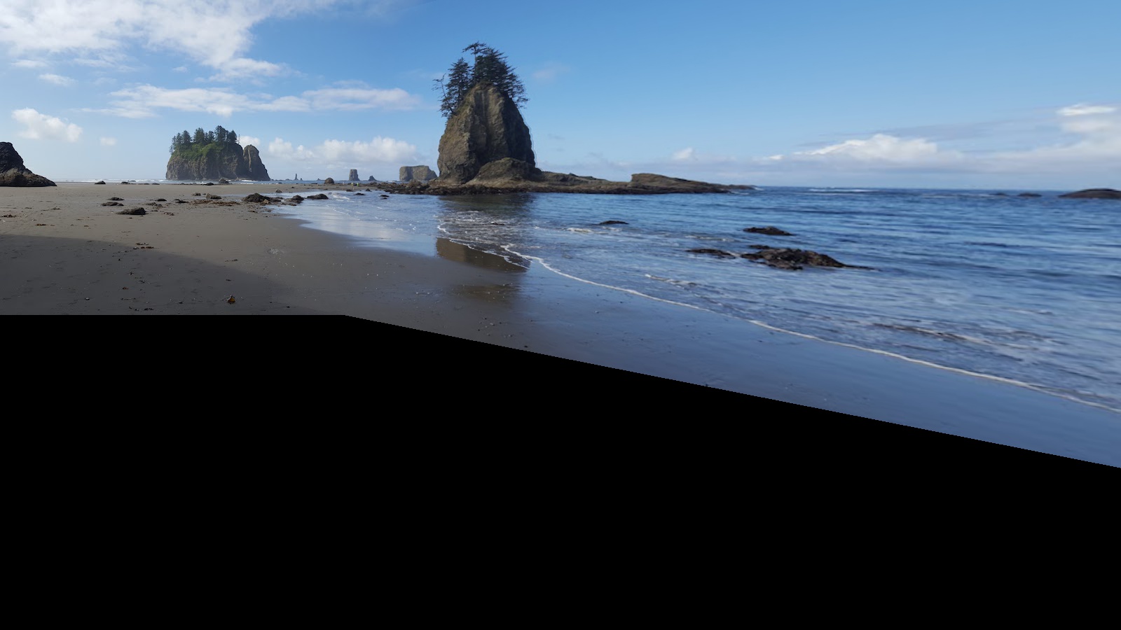
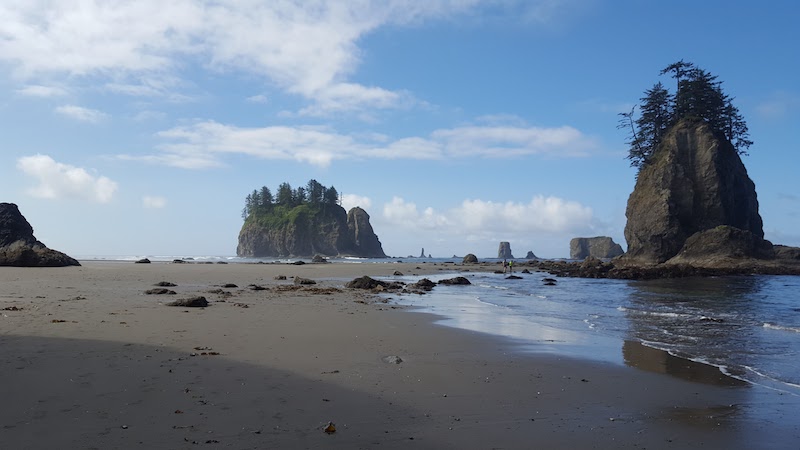 Original picture, left half of view of La Push beach in Washington
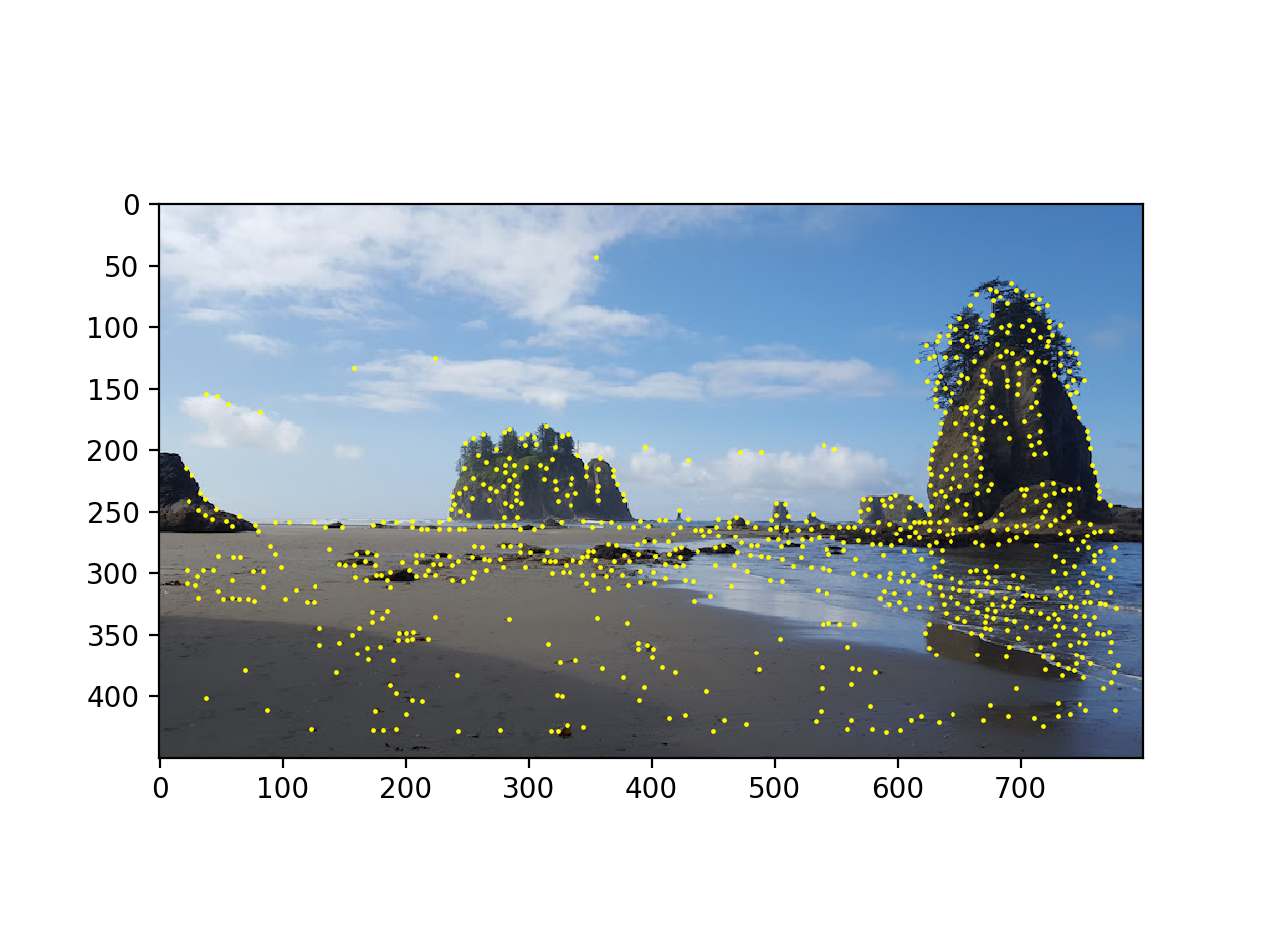
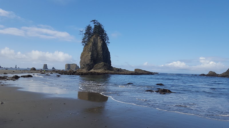 Original picture, view of right half of view of La Push beach in Washington
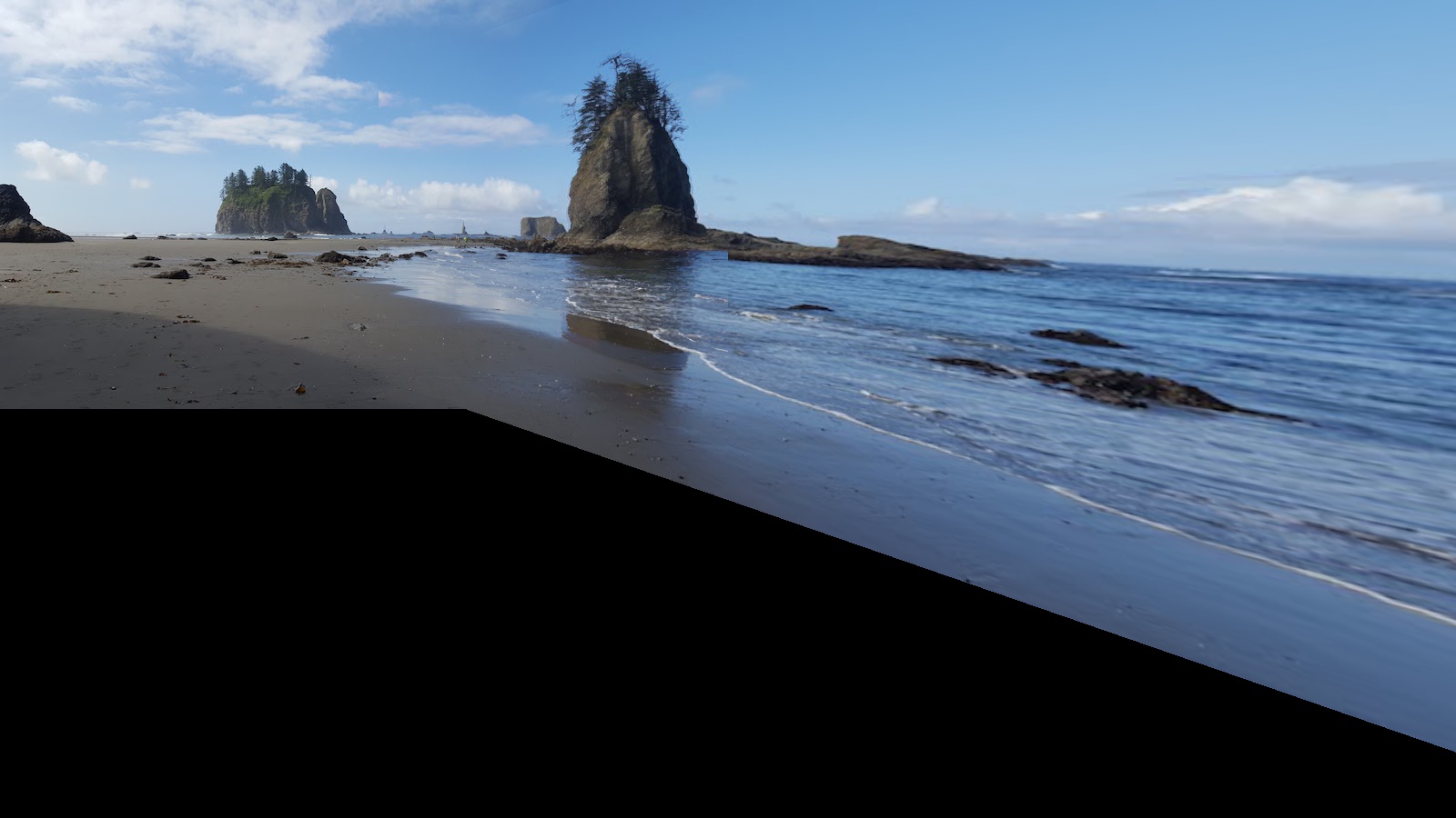 Combined image, using np.maximum to select pixels in overlap region.
Part B: Feature Matching for Autostitching
This part of the project is an adapted implementation of the paper Multi-Image Matching using Multi-Scale Oriented Patches by Brown, Szeliski, and Winder.
Part 1: Detecting Corner Features in an Image
This part of the project involved using a Harris Interest Point Detector to identify corners in images. Using the provided starter code, I was able to identify points in the image strong "h" values, indicating that those points were likely corners in the image. Running the starter code with slight modifications to the minimum distance between points and the threshold yielded the following results.
 Picture with Harris corners before thresholding
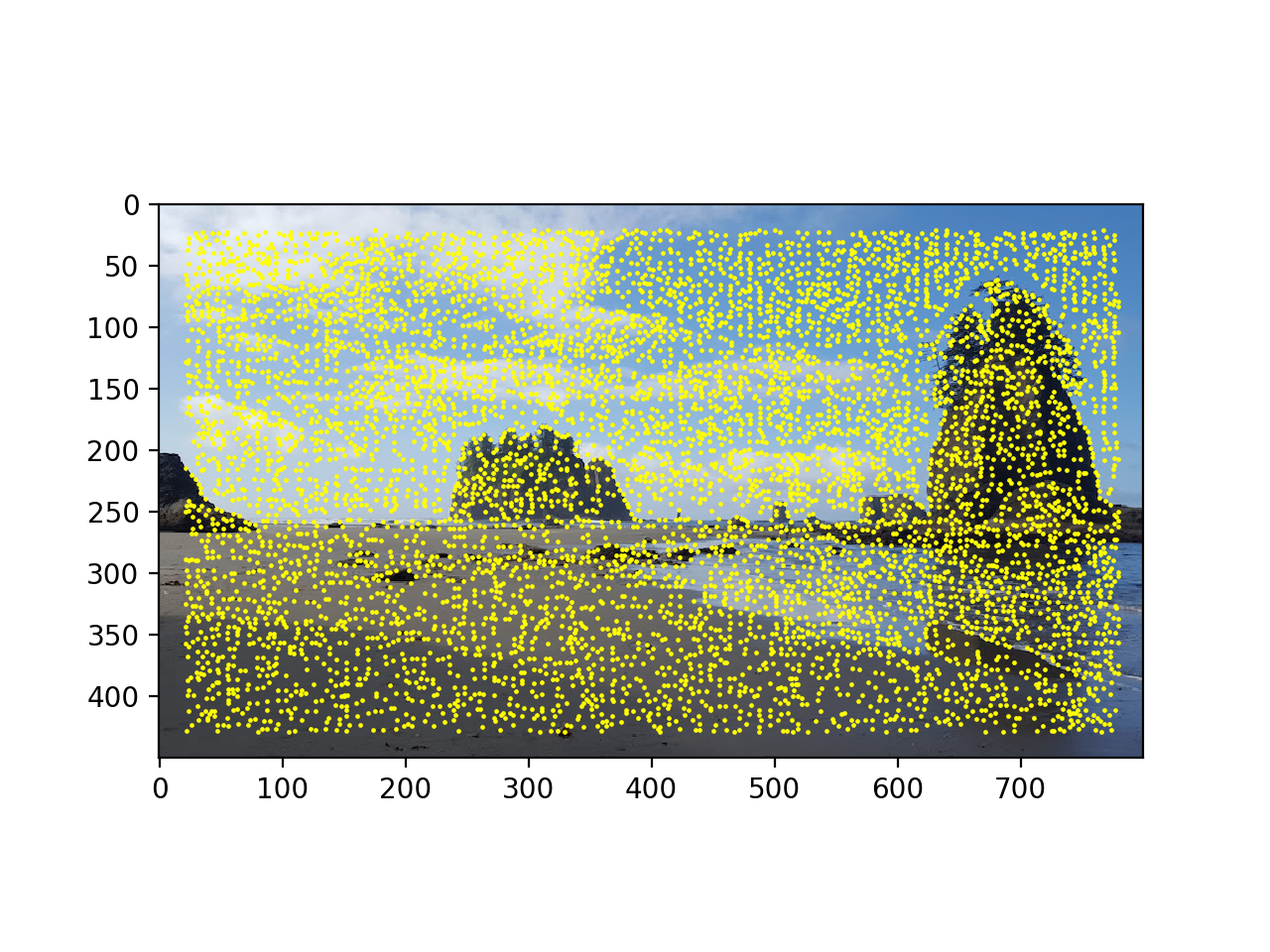
 Picture with Harris corners after thresholding
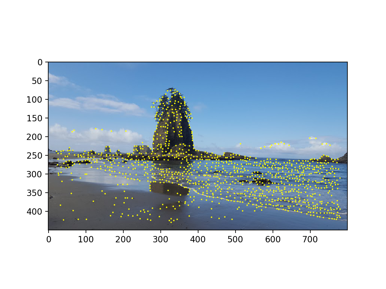 Other picture with Harris corners after thresholding
Part 2: Adaptive Non-Maximal Suppression
As shown by the previous images, the Harris corner code provided a large number of possible corner points to consider. We want points that correspond to the "best" corners but that are also more spread out over the picture. To do so, we implement the ANMS algorithm. This algorithm involves suppressing points based on their corner strength, and only chooses the maximum point within a radius. The minimal radius is calculated according to the formula:
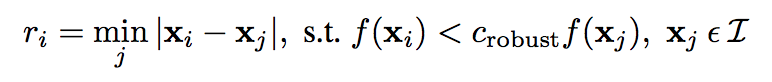
This claims that we can find the minimal radius by comparing the distance between two potential points, where the corner strength of the first is < 0.9 times the corner strength of the second (hyperparameters defined in the paper). Once we calculate these radii, we want to select the 500 points thta have the largest radii. These are then used in the next steps of the project. This algorithm output the following results:
 Picture with Harris corners after ANMS
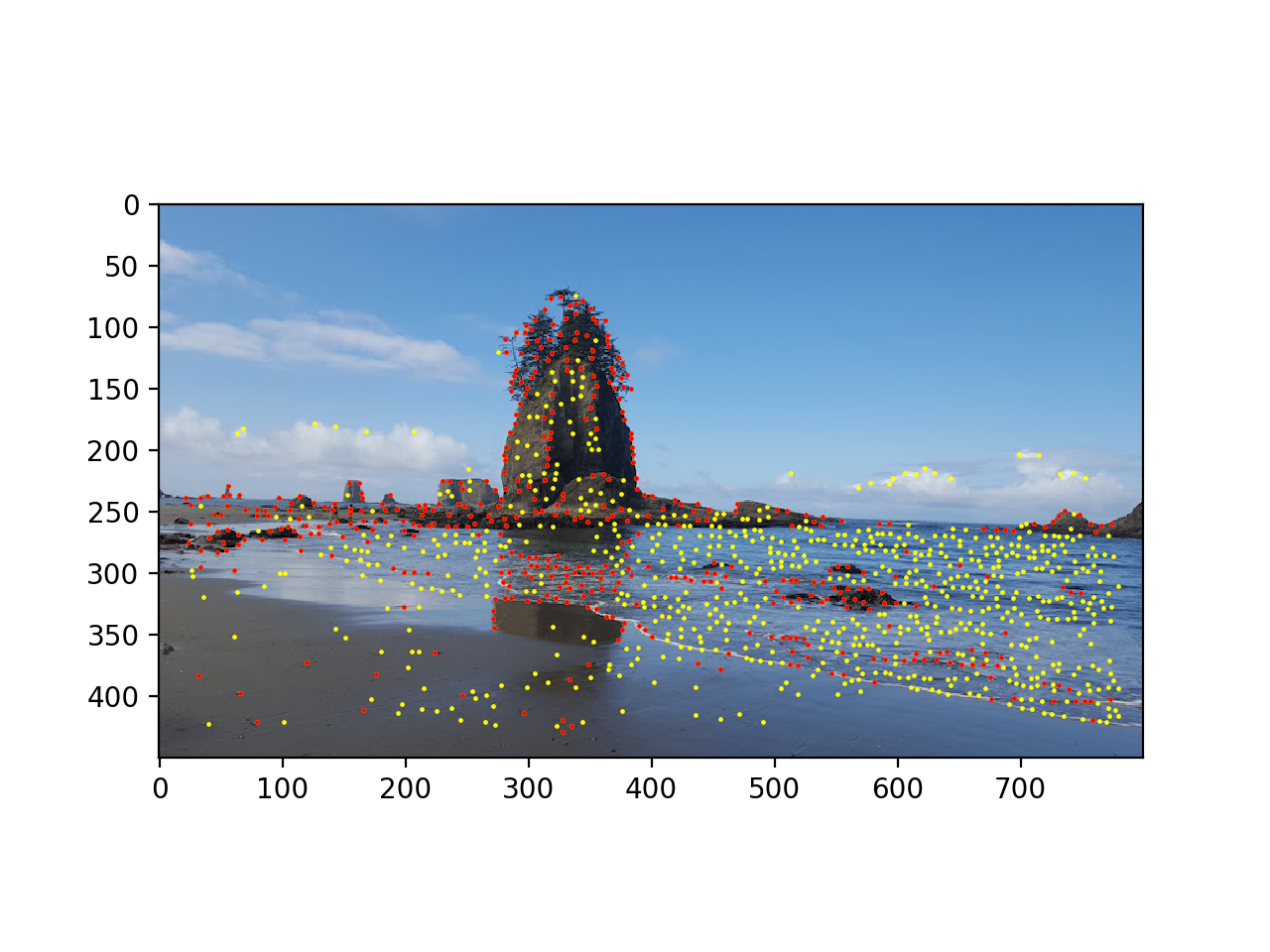 Other picture with Harris corners after ANMS
Part 3: Feature Descriptor Extraction
This portion of the project involved extracting a "feature" for each point found in the previous part. Features are 8x8 patches of pixels surrounding the point of interest, but sampled from a lower frequency than the interest points. To do so, we first take a 40x40 sized patch surrounding the point of interest, and then downsize it by a factor of 5 to produce an 8x8 patch. This method of sampling the image is intended to prevent aliasing. Once this 8x8 patch has been selected, we normalize it to have mean 0 and standard deviation 1. Doing so makes the patch invariant to affine changes in intensity (bias and gain). Example patches:
 Example feature patch extracted
 Example feature patch extracted
Part 4: Feature Matching
Now that we have identified features in both images, we want to find the ones that correspond. We do so by calculating the distances between all pairs of features using the provided dist2 code. Once we have this, we calculate the first nearest neighbor and second nearest neighbor -- those with the minimum and next minimum distances, respectively. We then use the Lowe method of thresholding based on the ratio between the 1NN and the 2NN. From the paper, we pick a threshold of 0.5 in order to pick correct correspondence points. This method resulted in identifying the following correspondence points:
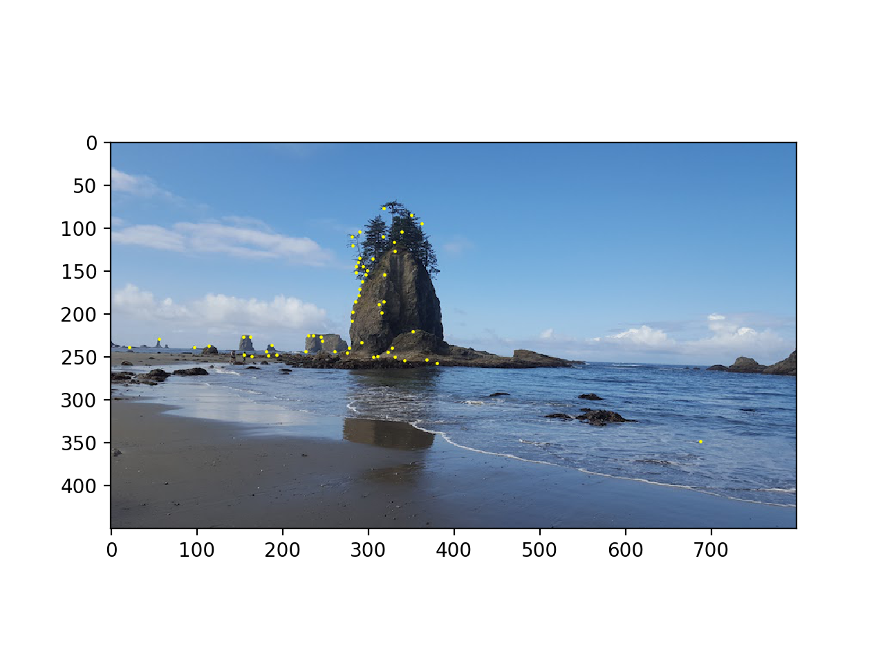
 Left image potential correspondence points
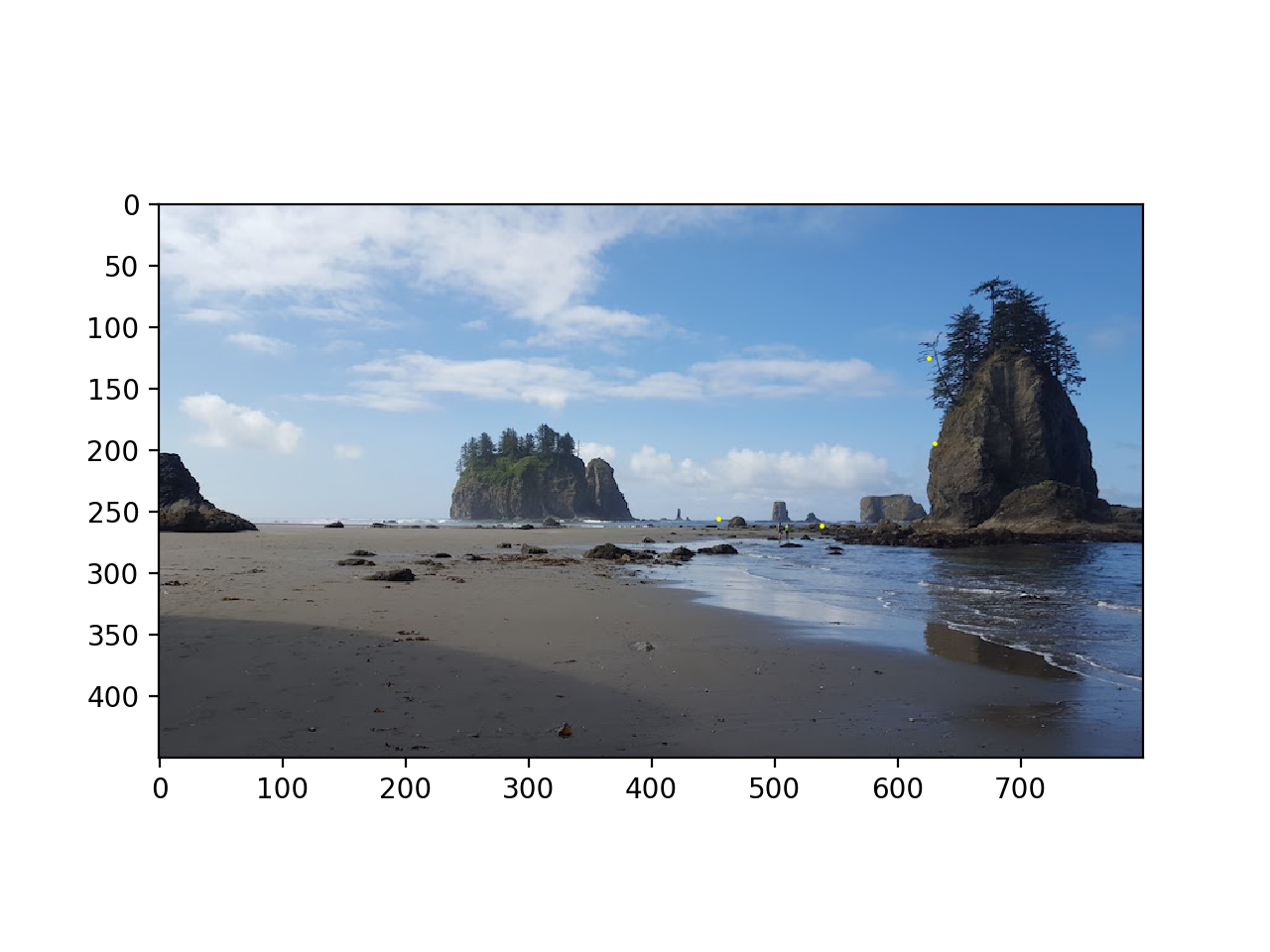
 Right image potential correspondence points
Part 5: RANSAC
Now that we have potential correspondence points identified, we have to find the ones that actually align. To do so, we implement random sample consensus, or RANSAC. This involves randomly picking four pairs of points, computing the homography matrix between them, then multiplying all the correspondence points by the computed homography and calculating the error between the predicted points and the actual defined correspondence points. We count the number of pairs that produce an error less than an epsilon of our choosing, and choose the homography matrix that yielded the highest number of "inlier" points where the homography produced a prediction within a suitable error range. The result of RANSAC produced the following correspondence points:
 Left image matching points
Right image matching points
Combining to a Mosaic
Reusing the warping code from part 1 produced the following images:
Manual warping
 Auto warping
Manual warping
 Auto warping
Manual warping
 Auto warping
What I Learned
I learned that you can do so many really cool image manipulations just by using homographies. I also thought it was cool to see how even though two images taken of the different portions of the same overall scene from slightly different angles may appear individually to be taken from the same perspective, but actually the objects in the image are warped slightly and is much more noticeable when trying to stitch the images together.