This is first part towards autostitching mosaics. In this portion, we will recover homographies from two different images and make sure that our image warping, rectification, and blending work well.

The goal is to eventually be able to stitch these two images together. This is my patio. I took the photos by standing in one place and rotating my torso, trying my best to keep the horizonatal aspect relatively the same.

Below are other viewpoints I wish to stitch together.

In order to able to warp the images and blend them, we must recover the homography between the two images. The homography is the transform between two projections, represented by 3x3 matrix, H. To find this matrix, we need 4 correspondance points, giving us 8 degrees of freedom. Our 4 correspondance points, represented by an (x, y) are being mapped to the correspondance points in the second image, (x', y'). Finding the transformation between a set of points p and another set of points p' comes down to setting up systems of equations and solving via least squares.

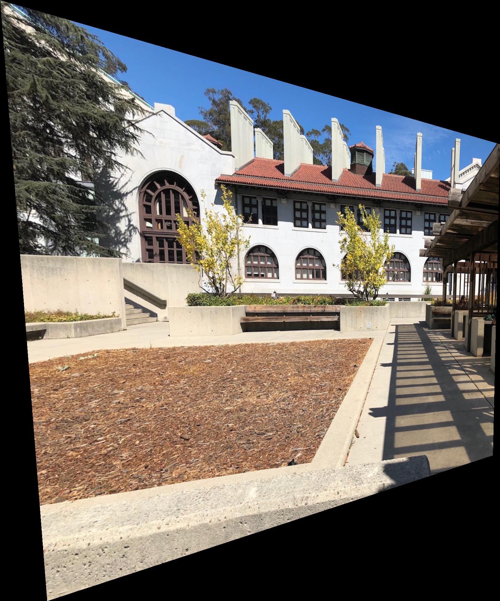
Now that we are able to recover homographies, we can start picking points and warping images. For my two images above, I picked 6 correspondance points each that outlines the corners of the wooden and brick buildings towards the center. The warping process is similar to one in proj4, where we apply the inverse homography, interpolate the colors, and then assign the colors. Below is the result of warping the second image to the plane of the first image.

Likewise, we can rectify images. This is where we take outline a square in one image, and project it such that it as forward-facing as possible with 90 degree angles. To do this, you take one image and select 4 correspondance points that outline a square in the scene. I then select 4 correspondance points on the same image, this time eye-balling a forward-facing square. In the image below, I outlined the bases of the right tree in the photograph. Below is the result of rectifying that image.

Below is a similar result of outlining the black square in the center.

In order to make a mosaic, we need to warp our second patio image to match the projection of the first, and then blend the result. I first calculated the size of the entire image. Afterwards, using the warped image I found earlier, I make a mask for both images and apply Laplacian blending. For these results, I only used a stack depth of 2, and there is still an edge that appears.

Notice, that across the center horzinal, the image seems continuous.

In the previous part, we manually chose the coorespondance points to which two images will use to stitch together. Now, we take the Harris Detector, Adaptive Non-Maximal Suppression, and the RANSAC algorithm to automatically configure correspondence points to stitch by.

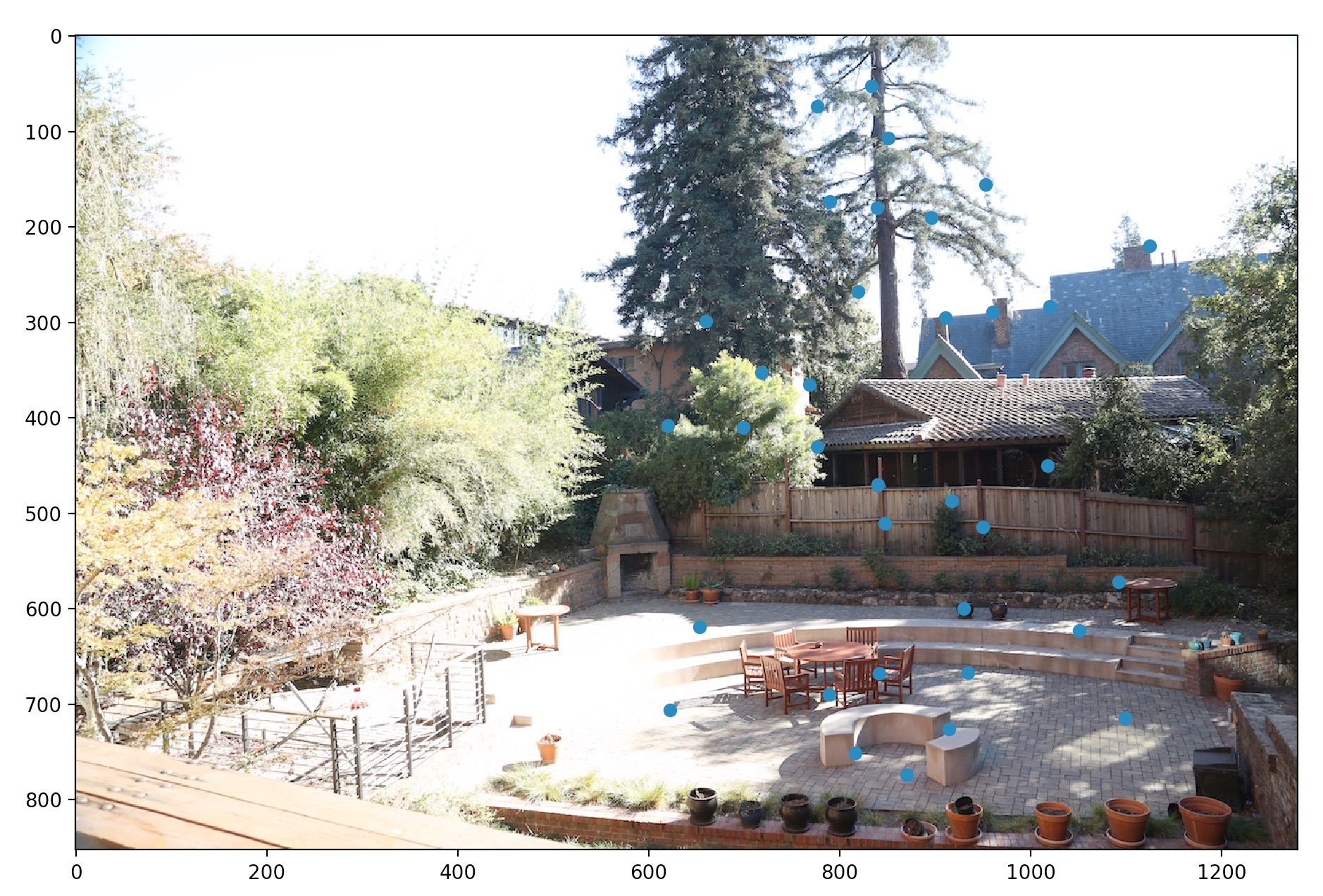
The Harris Detector is a known method for detecting corners in an image. It uses a combination of intesity operations to detect shifts in a window. For this project, we were given starter code, in harris.py to detect corners, which we can call interest points. One of the parameters was min_distance, which affected the number of interest points detected. I set this equal to 10 such that there weren't an excessive amount of interest points.

Below are interest points

We cannot use all of the interest points detected in both images to determine the auto-stitching. Our first step to determining which interest points are actually worth using, so we use a technique called Adaptive Non-Maximal Suppression. As the name suggest, it suppresses the amount of interest points by making sure they are evenly spaced. That is, we only consider interest points that are out of certain radius by their neighbors. The equation used is here.

c_robust is a constant set to 0.9, "which ensures that a neighbor must have significantly higher strength for suppression to take place" according to the paper Multi-Image Matching using Multi-Scale Oriented Patches. For my results below, I picked the 250 points with the largest radii.

Now that we have an evenly spaced set of interest points on both images, we then must determine which ones correspondant to one another. To do this, we need a way to describe an interest point, such that we can compare this description with another to see if they match. One way to do this is, for every interest point, make an 8x8 sub-sampled window corresponding to a window around the interest point. If two of these window descriptors match up, under a certain threshold, we can classify them as a point. Below are examples of these descriptors.

According to Multi-Image Matching using Multi-Scale Oriented Patches we can establish a threshold of considering two descriptors matching based on the first and second closest match. For a specific point in image 1, we compare its descriptor to every other point's descriptor in image 2. We keep track of the first and second closest match, call them 1-NN and 2-NN respectively. If the ratio, (1-NN / 2-NN) is below some threshold e, then we consider the point in image 2 that produced the 1-NN to be a match with the individual point in image 1. This threshold can be varied for different results and can be chosen by looking at figure 6B in the paper.

Below are the results of matching correspondance points. The threshold was set of 0.5 looking at the 250 interest points with the largest radii.

Below are also visualizations of the matching points.

The final part, now that we have matching points, is to again filter these points out and find the homography transform between the final matching points. We call this final set of matching points "inliers." The algorithm is given below.

We can choose the amount of iterations. For the results below, I used 5000 iterations, with an epsilon value of 0.5. Below are the visualized inliers used to find the final homography.

Let's compare the results from autostiching to mantual stitching.

Already, the edges around the trees in the center and patio in the center look a lot cleaner. If you were to do a horizontal wipe, the results from auto-stitching looks better.

Below are two more comparisons.

Notice the second gray car to the left. The seam is a lot smoother along that car.