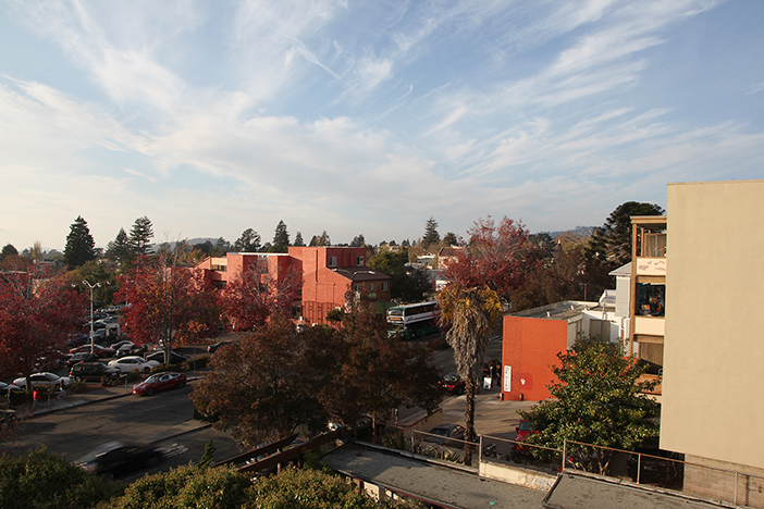
Panorama of Shattuck Ave.
CS 194 Project 6
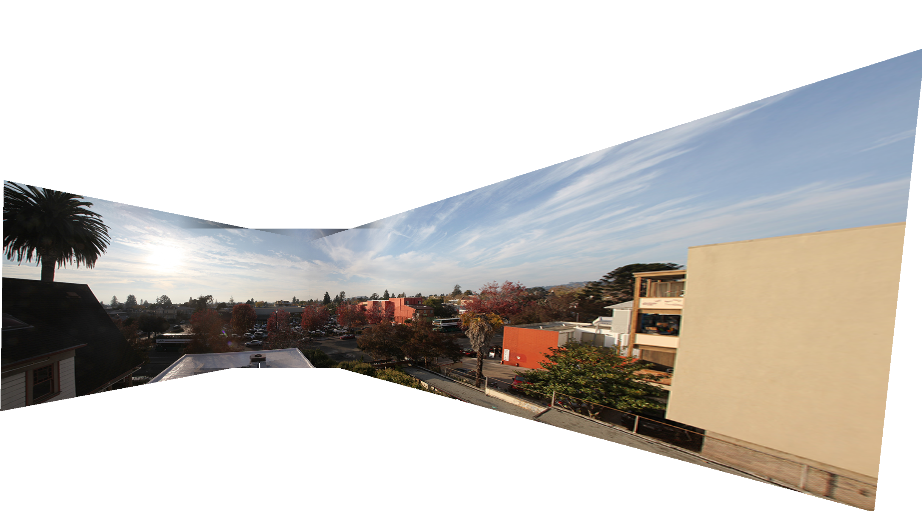
IMAGE WARPING and MOSAICING
By Stephanie Claudino Daffara
For this project I implemented creating panorama images by selecting correspondences by hand, autodetecting harris corners, and running RANSAC to estimate a homography, and finally a little bit of blending.
Rectification
The process of rectifying images was fun because it allows you to "align" pieces of an image to the perspective of the viewer. This way we can create the illusion that the image was taken from a straight on point of view. For all of these images selected the corners of the "object" that I wanted to rectify manually and warped it to a square or rectangle for the output.
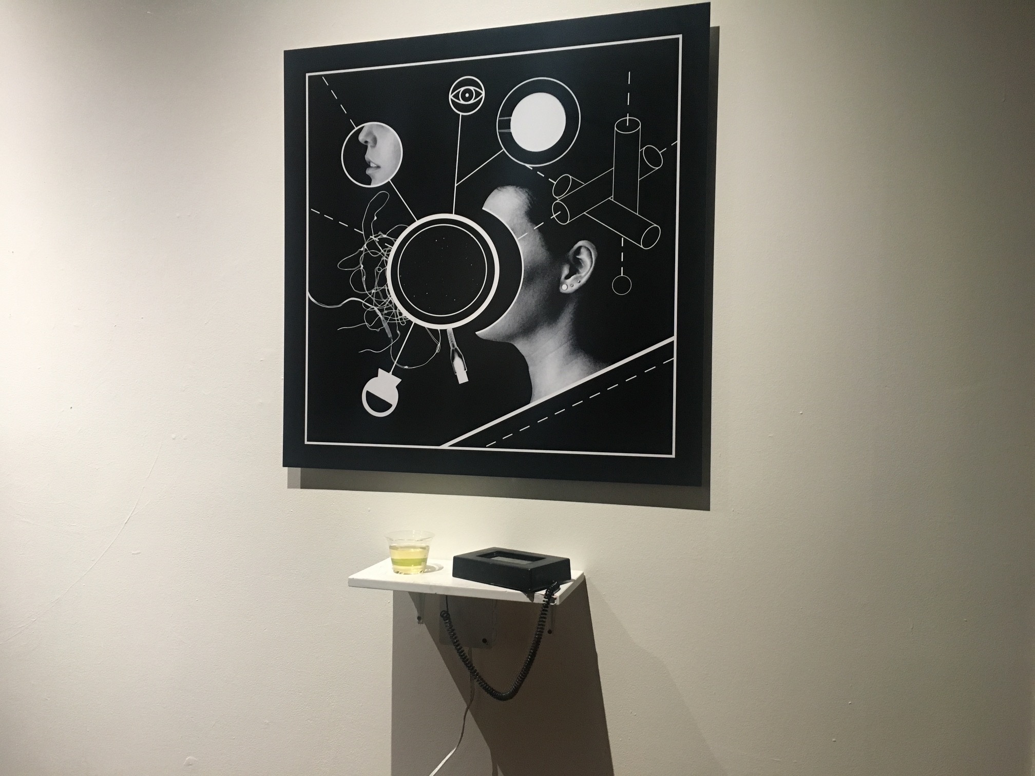
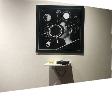
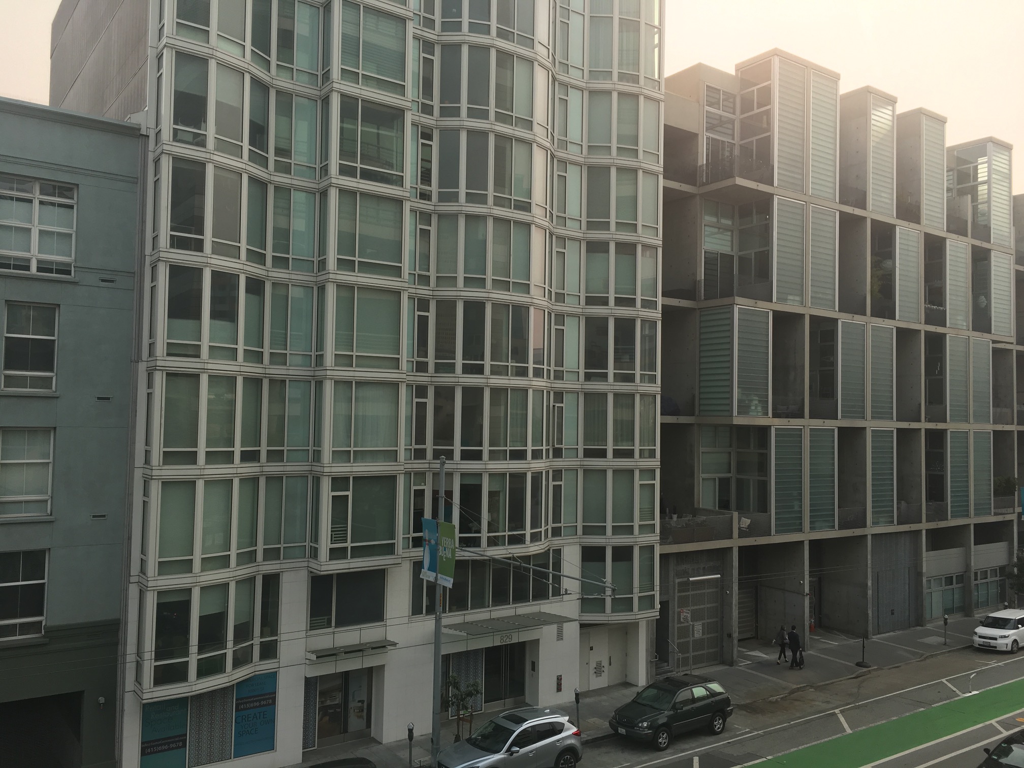
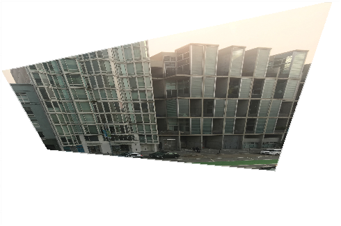
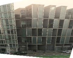

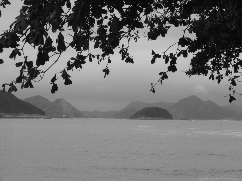
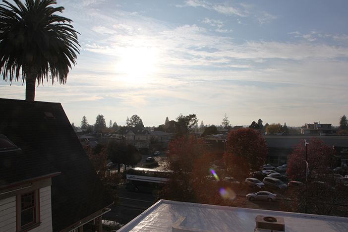
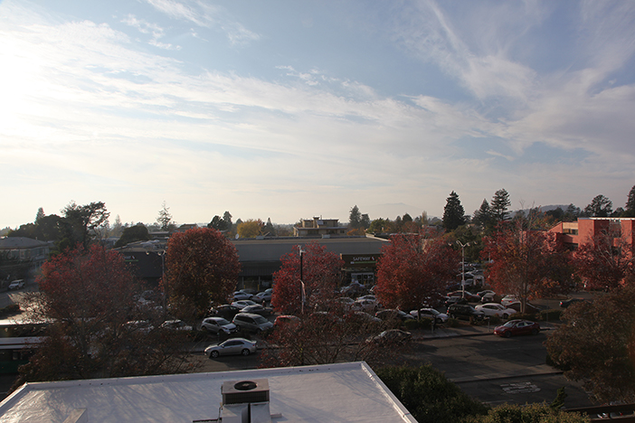
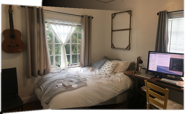
Image Stitching
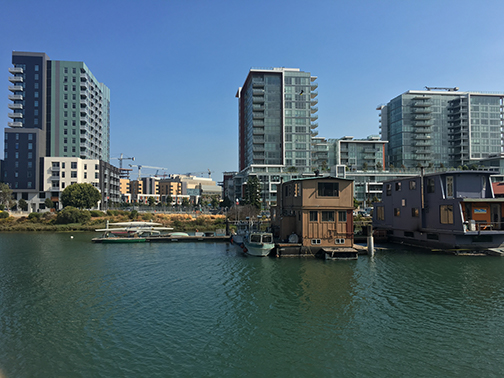
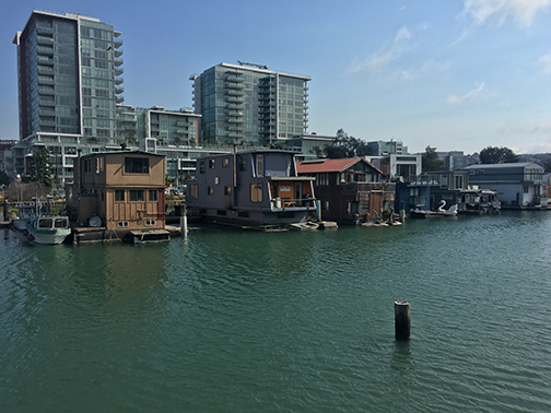
To create these panoramic images I took pictures without changing my center of
projection, and then manually selected the corresponding points. On average I selected about
10 interest points. Once I had my corresponding points, I then computed the homography between
both images by solving for Ah = b where h is a column vector of
8 unknowns. Once I recovered the homography I warped the source image to the destination image by
multiplying H and my source image's corners, and then interpolated for every
other point in between. Finally, I paste both images on top of each other, with the proper displacement
and blend the seams. I used a gradient mask to blend the images. I also tried using the laplacian
pyramid for blending but ended up with very similar results.
Feature matching for Autostitching
For autostitching I followed this paper with some simplifications. The task was split into four steps: Detecting Harris interest points, implementing Adaptive Non-Maximal Supression, implementing feature descriptor extraction, and finally feature matching. Once I found matching features I simply used the homography, warping, and blending function I had already implemented.
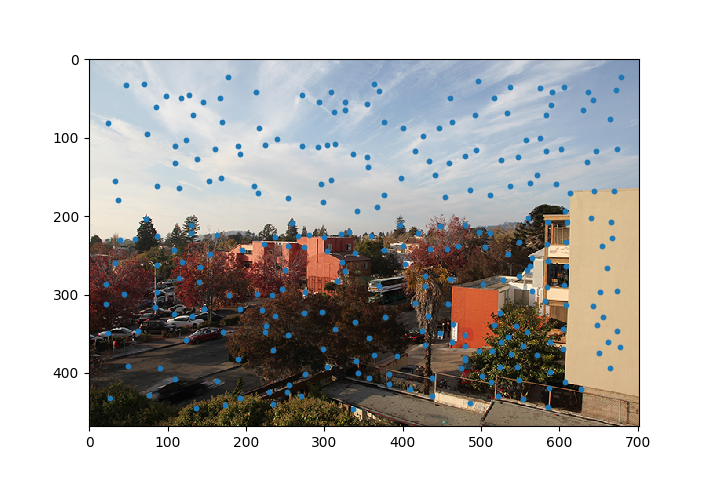
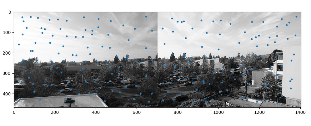
Harris corners
A Harris corner detector essentially convolves a window over the image and at each pixel shifts it in different directions. Shifting a window in any direction will give a large change in intensity, unless there is a corner within your window. Below I demonstrate an image with its Harris corners.
Adaptive Non-Maximal Suppression
Here I implemented Adaptive Non-Maximal Suppression in order to reduce the number of corners that the Harris detector found. In the following image I set my cap on 200 points. The impressive thing about this algorithm is that it selects mostly evenly spaced out points so that the homography computed later is not bias to a single section of the image. The way this works is by selecting points that have "strong" points (as determined by the Harris detector) furthest away from themselves. This way we select points with the biggest possible radius and keep reducing the radius around them until we reach the desired number of interest points. Here is an image displaying the ANMS points for both source and destination images. Please note that I did not use these 100 ANMS points in the rest of the algorithm, I reduced the number of points desired here to make it more clear that although there are less points they are still spaced out. Usually I would set my number of points to 200 or greater.
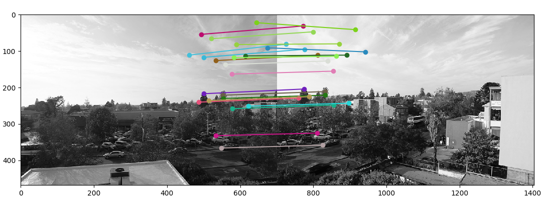
Feature Descriptor and Matching
Next I created 41x41 patches over each interest point and rescaled them down to 9x9.
I decided to use these sizes so that I could end up with a center pixel for my interest point. Then I used these
smaller patches as a feature descriptor to compare between both the source and destination images. Then I computed
the distance between each pair of patches between the two images and selected the ones that had a distance of less
than some threshold. For this image the threshold was 0.5. The following image shows the selected
matched feature points.
RANSAC
Finally in order to combine the images into a panoramic image I used RANSAC, Random Sample
Consensus to compute a robust homography estimate. Like most magical algorithms in computer science,
this one uses randomness to find the approximate best points to compute a homography off of. What it
does is selects 4 matches at random, computes the inlier points, and if I end up with more inlier points
or the same number of inlier points but a better loss score, then I keep those inliers as the current best.
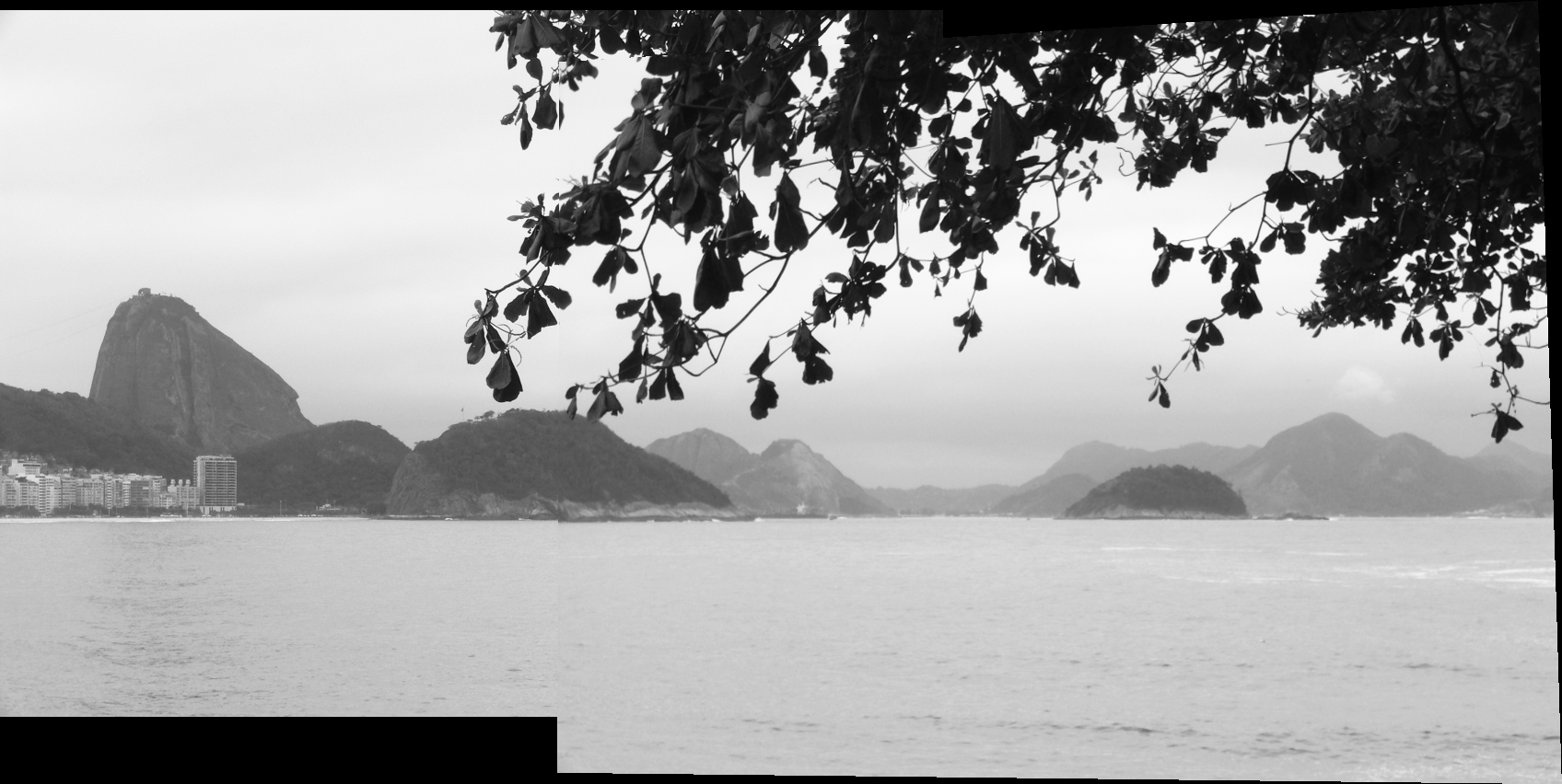
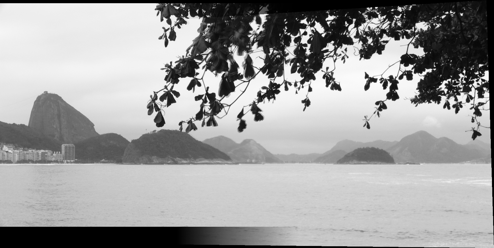
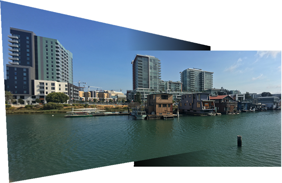
By doing this some k number of times I ended up computing the following panoramic pictures.
For these last two panoramas I did not get the auto-blending quite right yet. I tried using pyramid blending but the results are what you see here. With more time I would explore blending in the y-axis as well, which seems to not blend properly.
Learnings
I learned that homographies are basically projections. They are cool to work with and more powerful than I had expected. Rectifying images was very fun. I also believe that my pyramid blending did not achieve the results I would have expected (not that much better than simply copying and pasting the warped image on top of the other image). I'm not sure if this just the case for these images or if maybe there are some improvements that could be done to my pyramid blending parameters.
❤