Project 6 : [Auto]Stitching Photo Mosaics

Dorian Chan - aec

Part 1: Image Mosaics

Recovering homographies

If we have correspondences between two images, we can compute a homography matrix that provides the transformation between one image to the other image. We basically solve for the homography matrix using least squares, trying to match our input points in the input image to our specified output points in the second image.

Warping using the homography

Using that homography, we can warp the first image to the second image, and create an image mosaic! We perform inverse warping, where for every pixel in the output warped image we apply the inverse homography to get the source pixel.

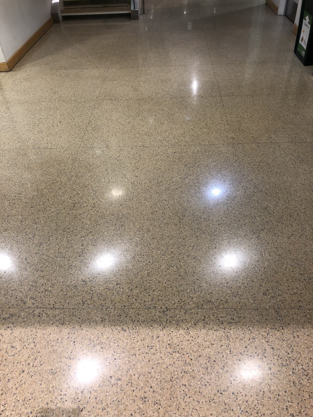
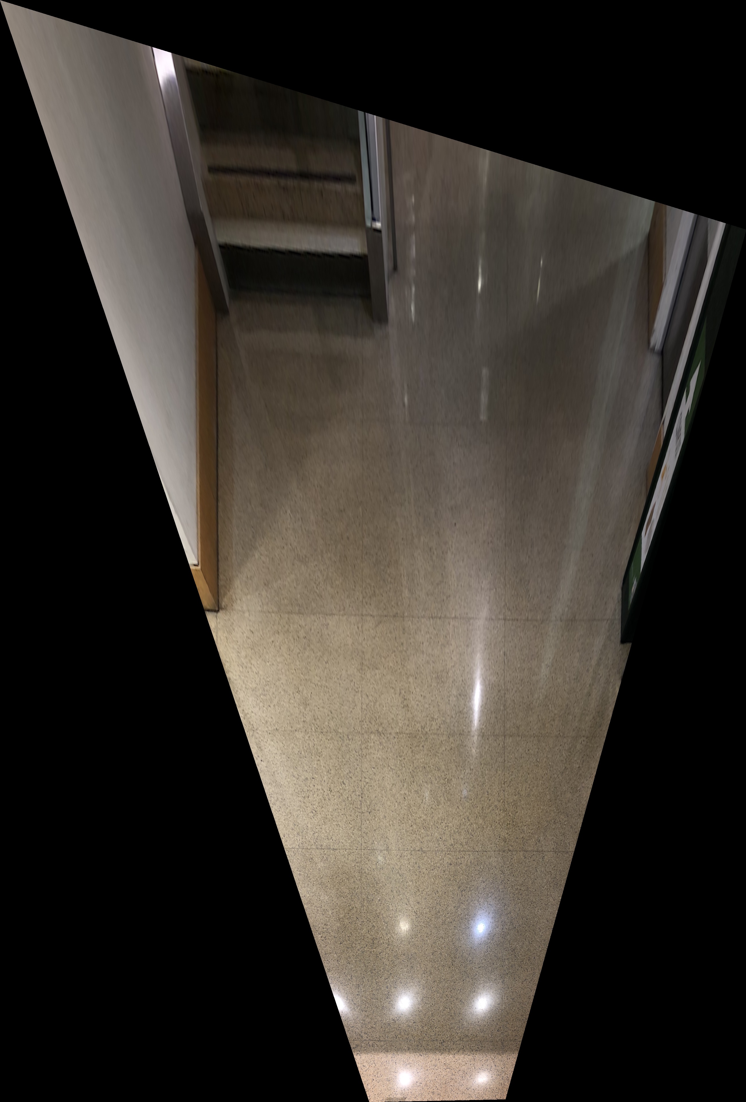
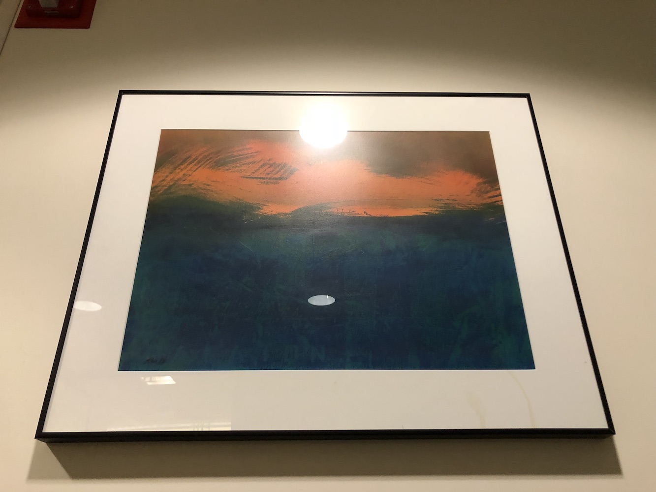
We can use the above warping process to rectify images, for example to change the perspective of an image. Here are a couple examples, that I took myself:

Pointing camera to look down at floor

Input:

Output:

Pointing camera to look straight at painting

Input:

Output:

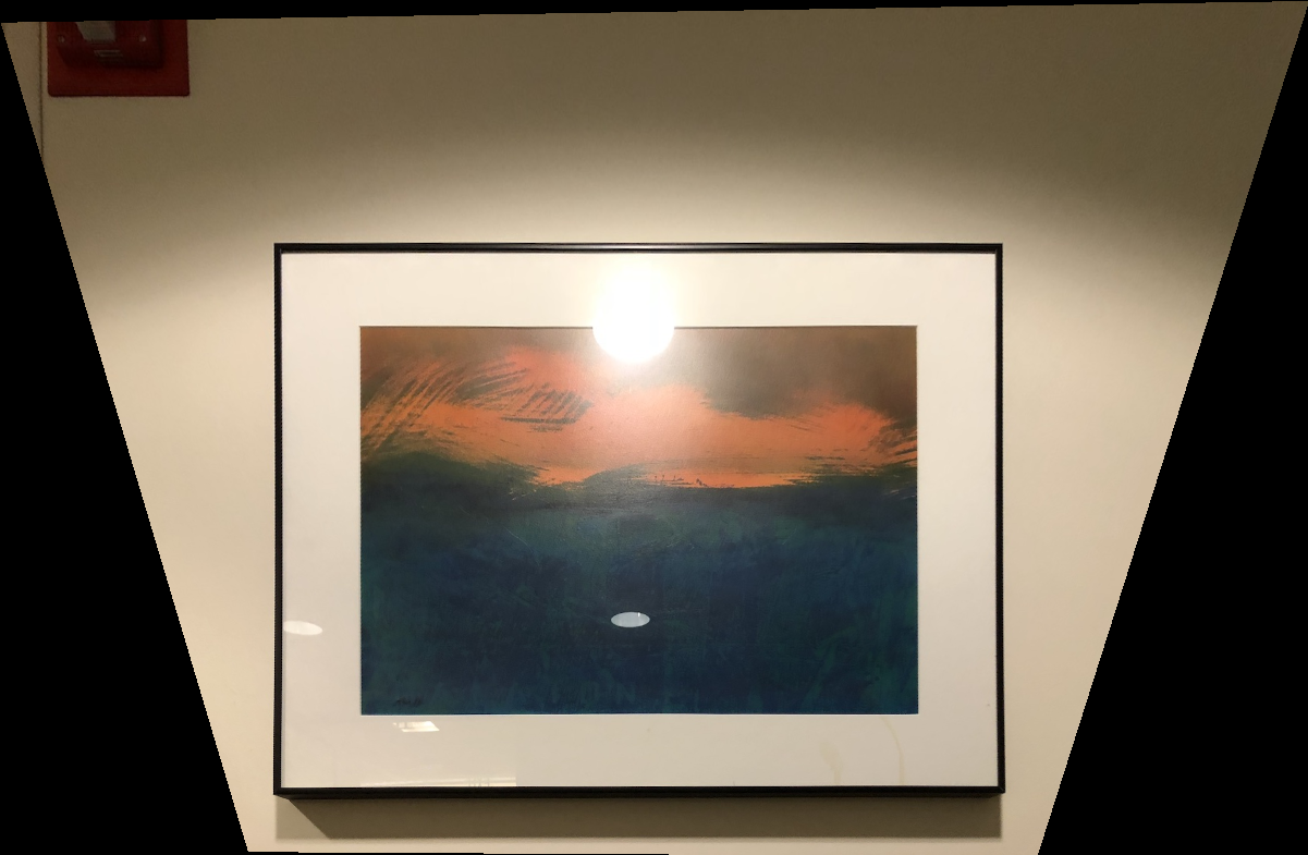
Image Mosaics

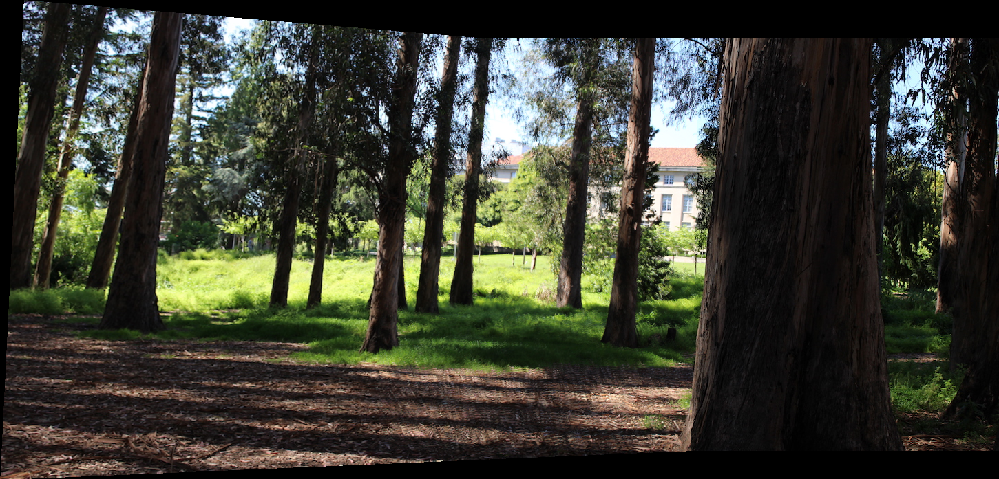
Here are some examples of image mosaics, where I combine a left and a right image to one output. I warp the left image to the right image’s plane. I use Laplacian blending to ensure boundaries look smooth, using a mask slightly smaller than the warped image.

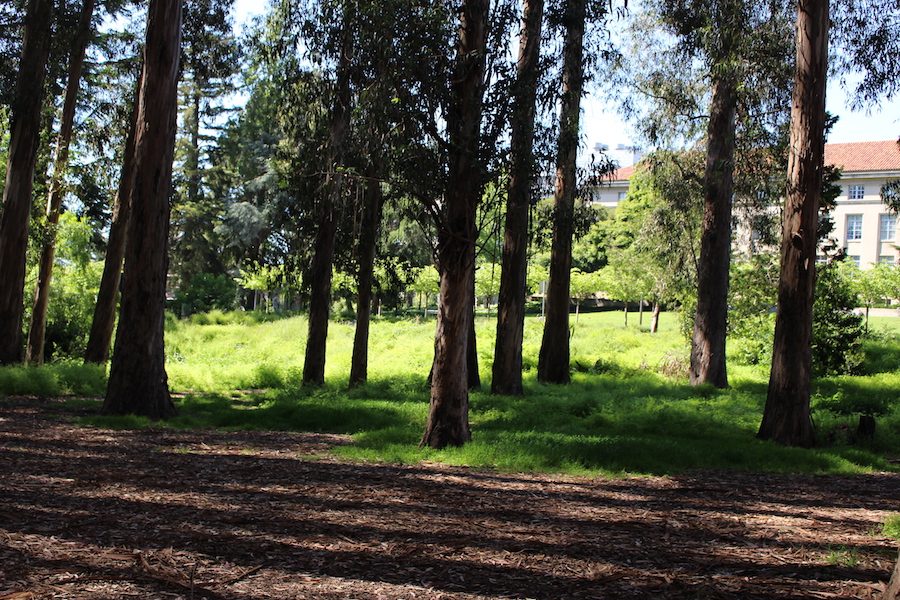
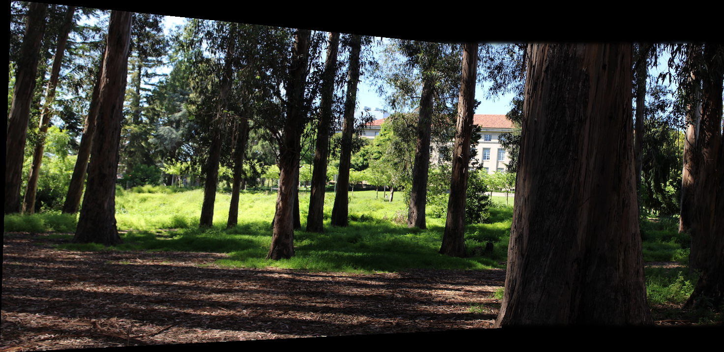
Eucalyptus Grove

Left:

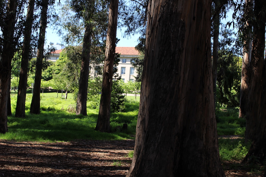
Right:

Output:

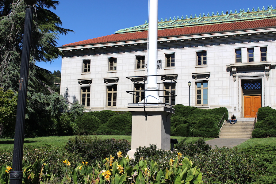
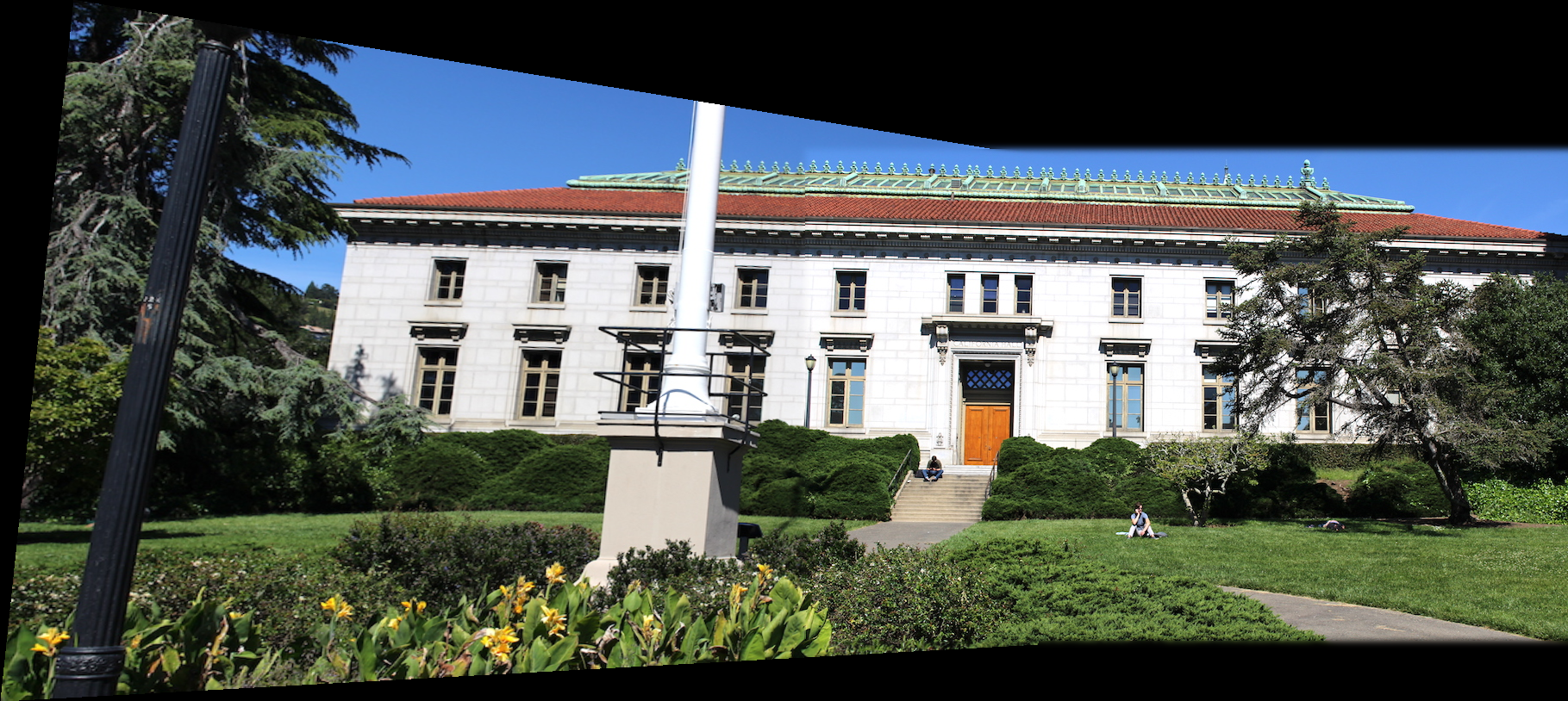
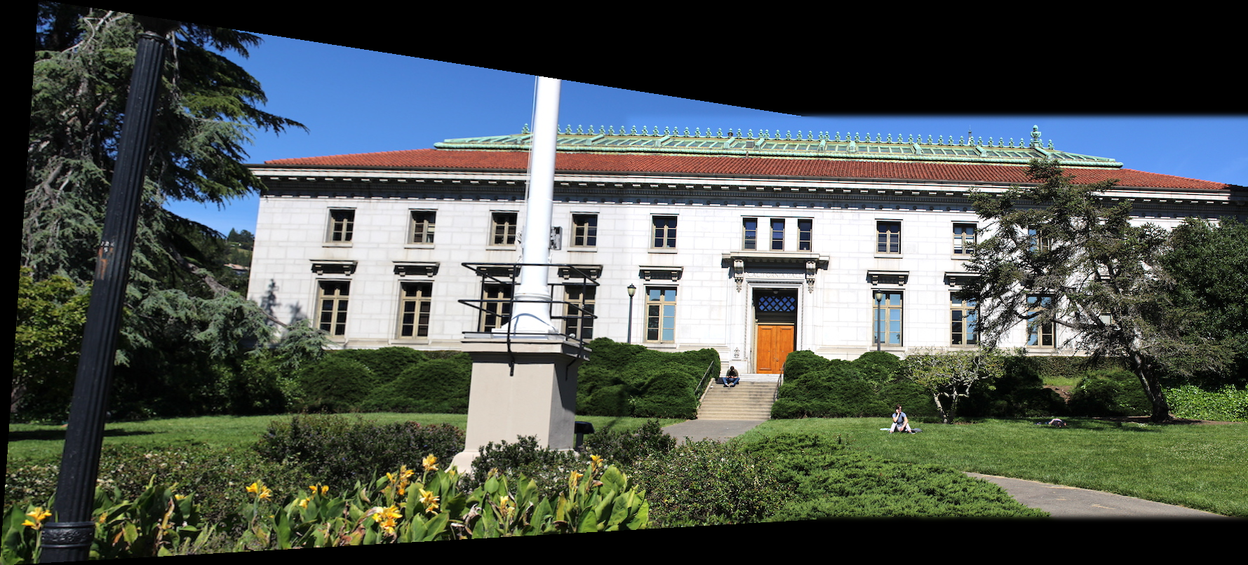
California Hall

Left:

Right:

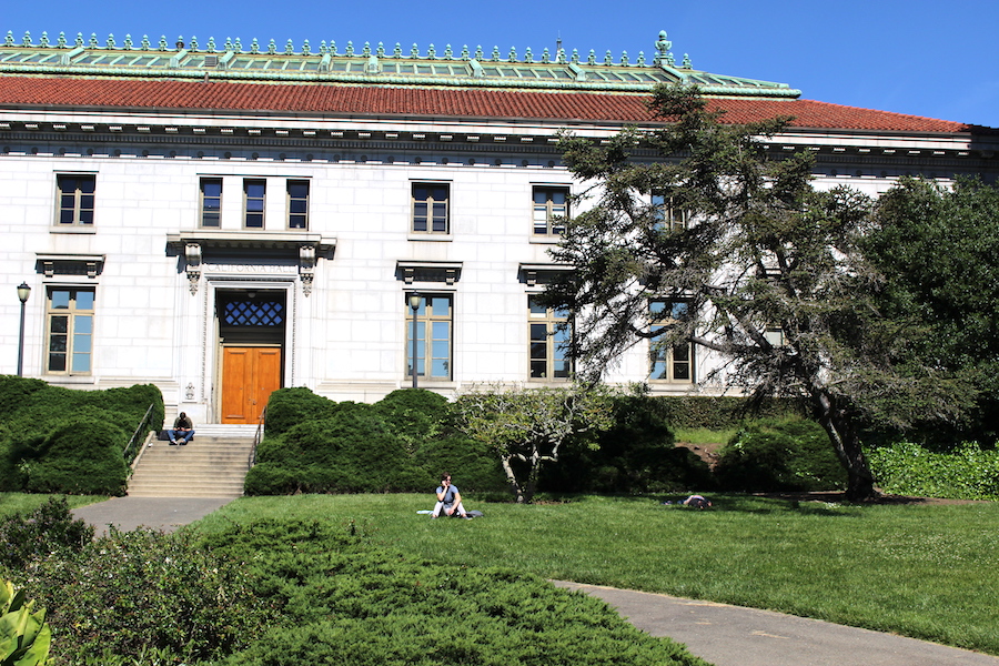
Output:

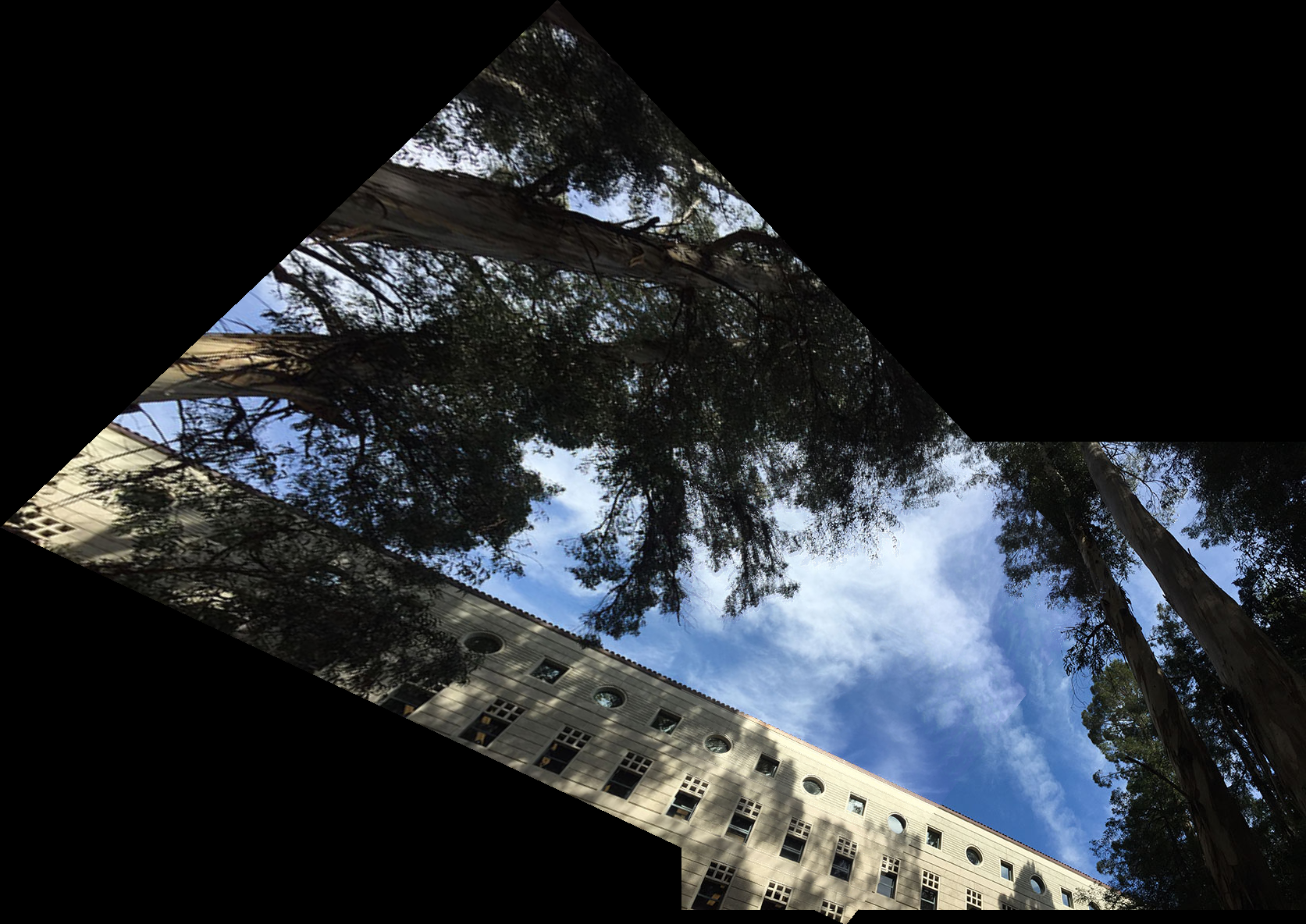
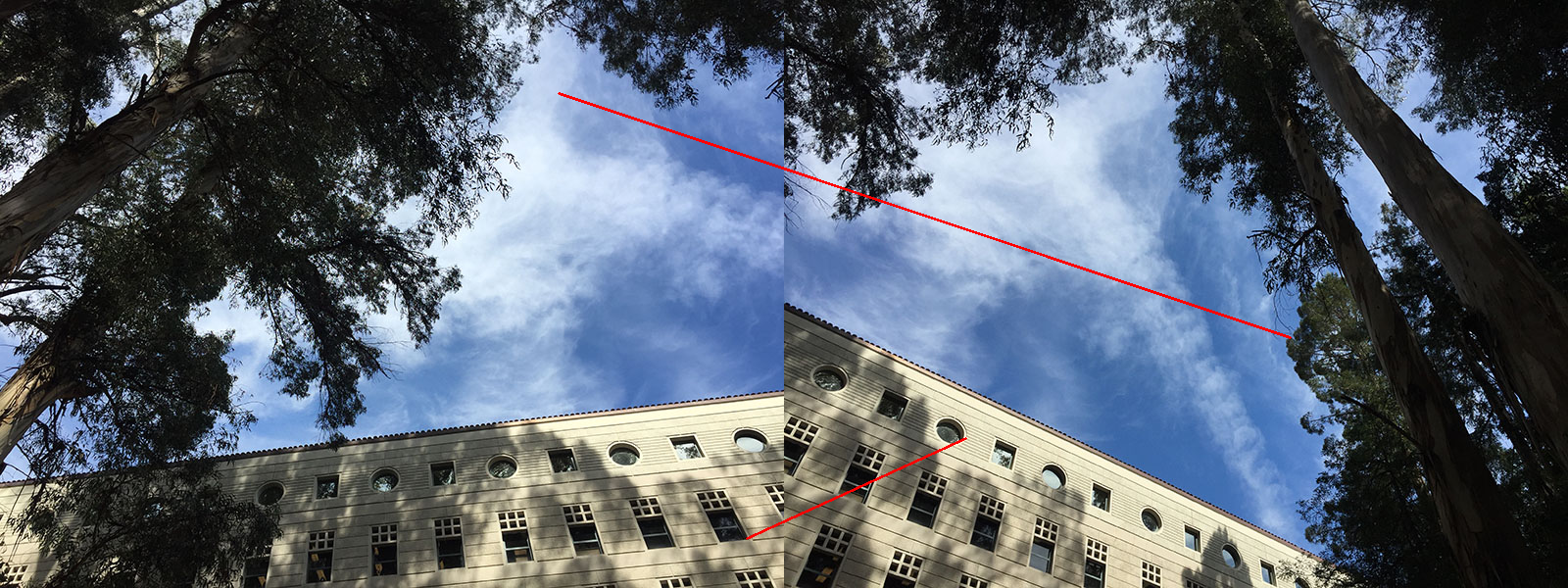
Sky Trees

Left:

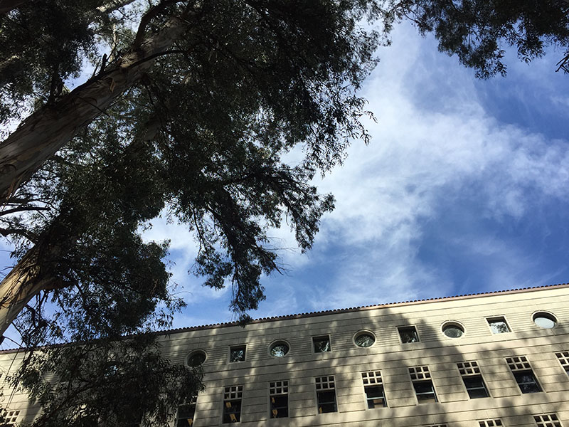
Right:

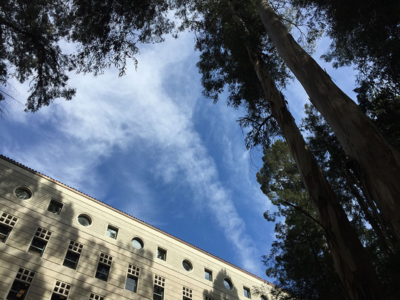
Output:

Part 2: Feature Matching using Autostitching

With the above in mind, how do we actually come up with the input correspondences? Before, we came up with them by hand - how do we do that automatically? We use a process called Harris Corners, MOPS feature extraction, and RANSAC to do this.

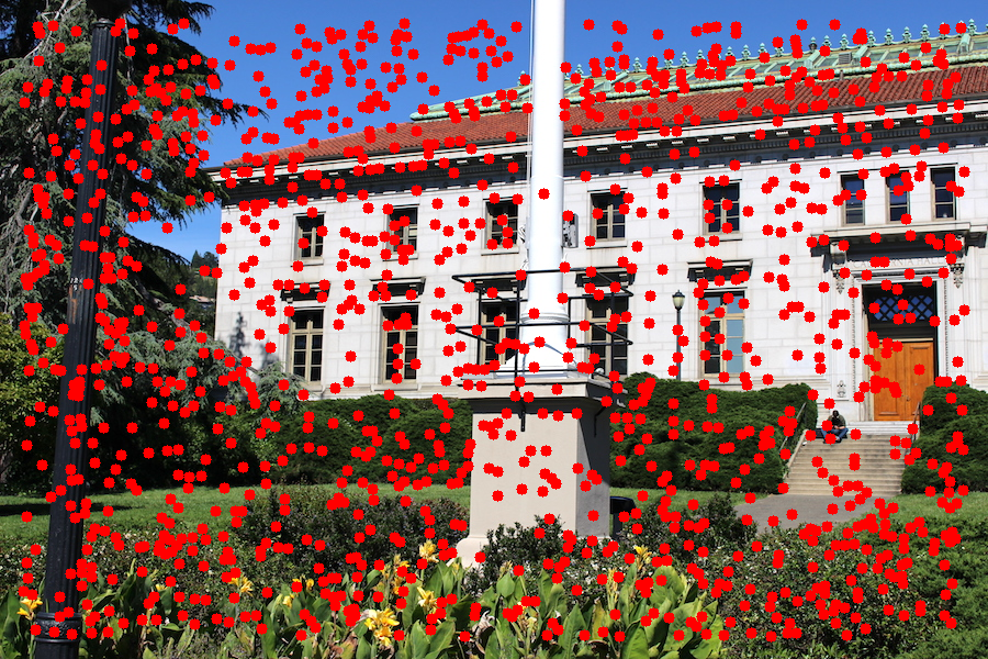
Harris Corners

The very first step is to detect features of interest in each image. We can use an algorithm called Harris Corners, which uses an eigenvalue process on a matrix composed of the gradients of the image in order to determine which pixels are important features. To demonstrate, here are some randomly selected Harris Corners overlayed over a test image.

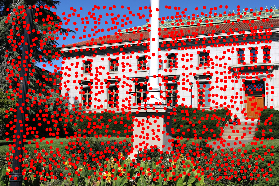
ANMS

One thing you might notice about the above is that some of the features are very bunched up, and some features are very far apart. Ideally, we’d like our features to be fairly evenly scattered about the image, to ensure that we can match over large portions of the image for our correspondences. To do this, I implemented an algorithm called Adaptive Non-Maximal Suppression, or ANMS, that attempts to evenly distribute the features. The basic idea is that the program orders features based the size of the radius in which that pixel is the biggest pixel. To spread out features, we want to select features that have very large radii, as when all the features have large radii they will be evenly spread out (they push and jostle each other). Here are some results. As you can clearly tell, this image’s features are much more spread out and not jumbled on top of each other, compared to the previous randomly selected features displayed above.

Feature Descriptor Extraction

Once we’ve actually found these features, now we have to get some information about the features in order to perform matching later - feature descriptors. In this case, we ignore rotations, and focus on axis aligned descriptors only. We essentially sample a 8x8 patch from the 40x40 neighborhood surrounding each feature - we sample on a low frequency, low passed image because small pixel shifts and rotations disappear at lower frequencies. Thus, using these low resolution neighborhoods our matching will be much more robust.

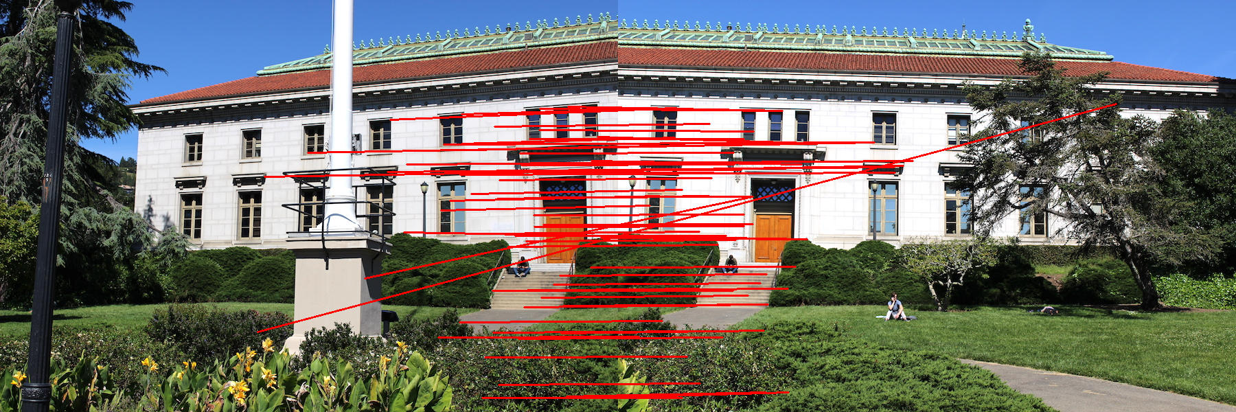
Feature Matching

Using these descriptors, now we can actually build correspondences between two images. The easiest way is to simply find the nearest neighbor in the other image for each feature in the current image. However, doing this can be very noisy - to fix that problem, we basically apply a process where we only select matches where the first nearest neighbor is much more similar to the input feature compared to the second nearest neighbor - that way we don’t select confusing matches that might throw off our later calculations. Here is an example of this applied algorithm on the California Hall dataset from above.

RANSAC

However, as you can tell from above, that process still isn’t quite enough to eliminate all of the bad correspondences. We need something more robust, which is why we use RANSAC. In RANSAC, we basically repeatedly try computing homographies using just the minimal 4 points, and seeing how well that homography works for all the keypoints and features in the two images we are using. We select the homography that works for the most features - we effectively do outlier rejection. Here are the same image mosaics from Part 1, now using RANSAC plus all the above Part B features. As you can tell, the seams are even less noticeable than Part A.

Eucalyptus Grove

Manual:

Automatic:

California Hall

Manual:

Automatic:

Sky Trees

This is a failure case. Basically, the left and the right image of this dataset involve rotation - as I mentioned before, we assume rotation invariance. Thus, our automated algorithm finds only two matches, which is not enough to generate a homography.

Matches:

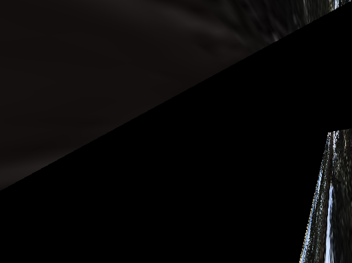
Output:

Manual:

What have I learned?

I think the coolest thing that I took away from this project is that sometimes algorithms don’t work with real life data. While theoretically the algorithm is perfect, real life data is inexact and buggy, and leads to a whole bunch of issues. As a result, we have to do a whole lot of robustness algorithms in order to get around that issue, i.e. RANSAC and the 1st/2nd nearest neighbors calculations.