Part A
Introduction
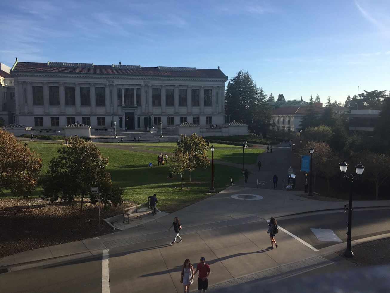
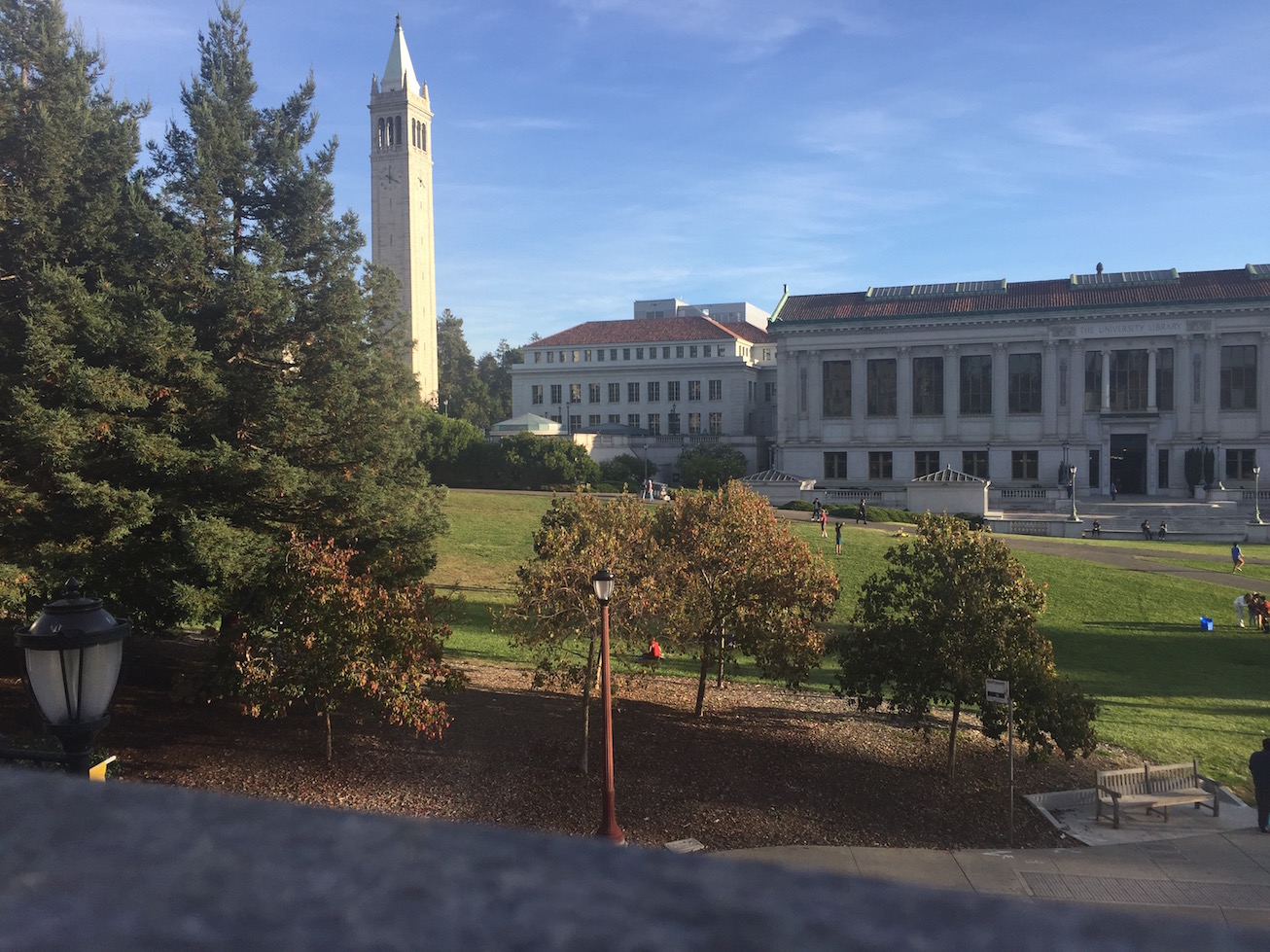
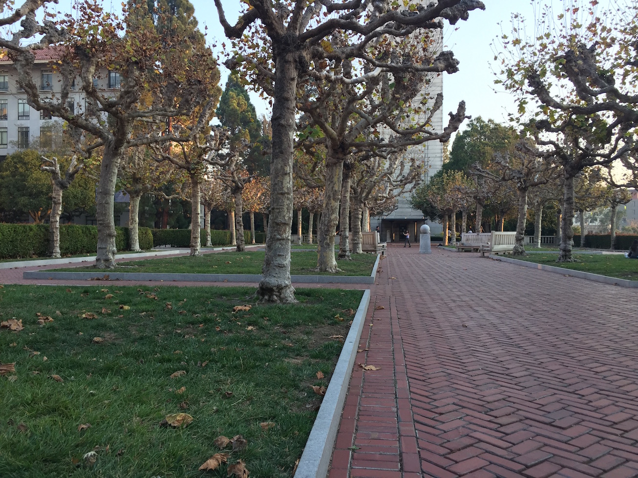
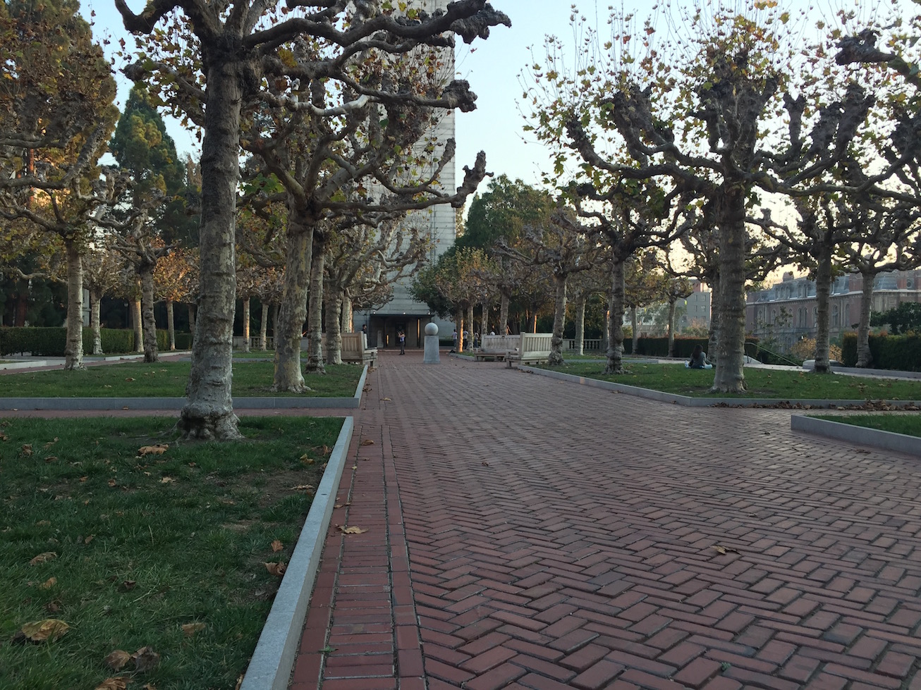
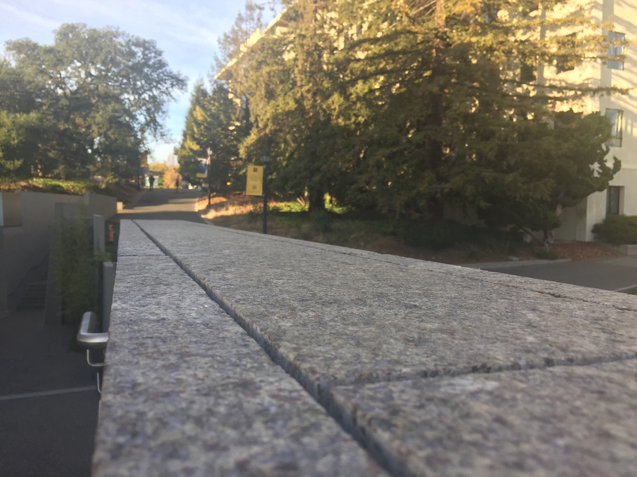
In this part of the project, we create panoramas from multiply photos by using the homography transformation to rectify images in the collection to a singular perspective, and then we blend the images together to create a panorama. Most images here were taken by myself on UC Berkeley's campus.
Recover Homographies
To obtain the homography matrix, we manually label corresponding points between images, and then use least squares to calculate the elements in the homography matrix. We formulate the homography matrix transformation into a least squares problem to do so, solving for a through h in the homography matrix, as i is already known to be 1.
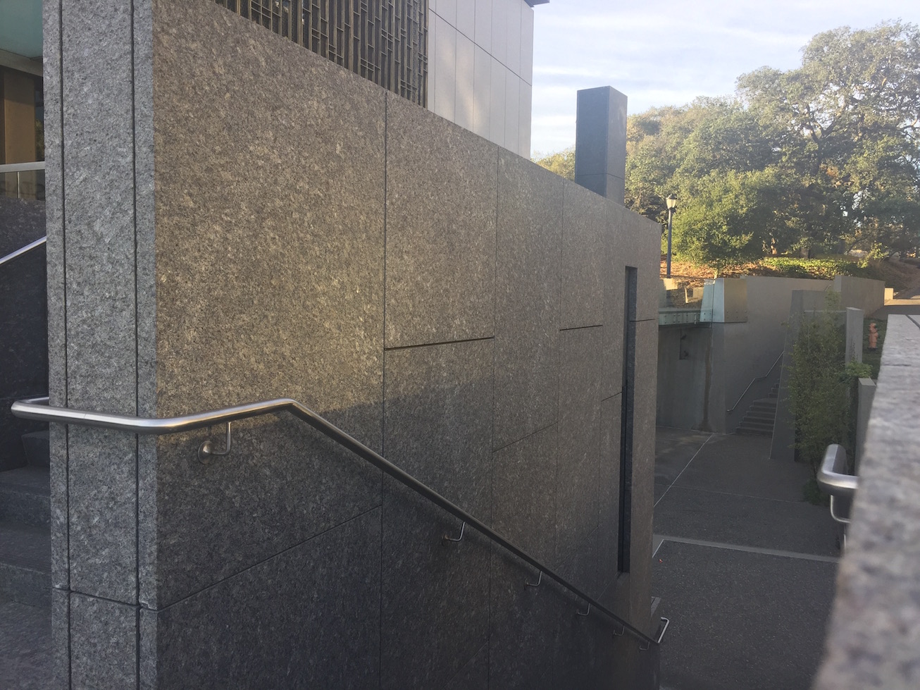
Image rectification
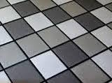
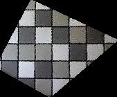
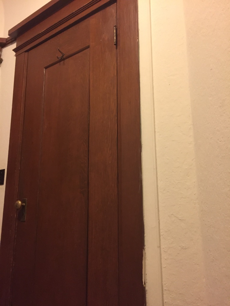
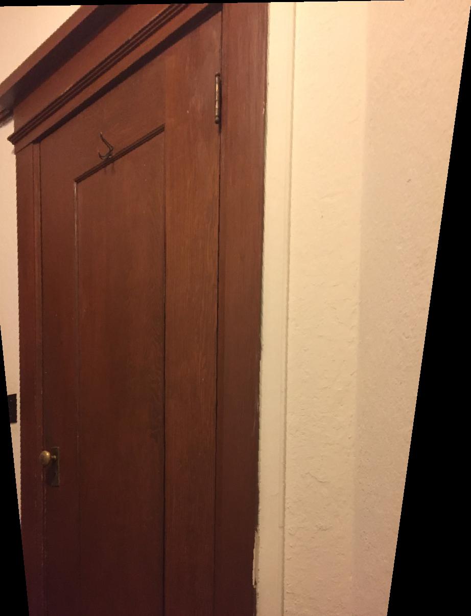
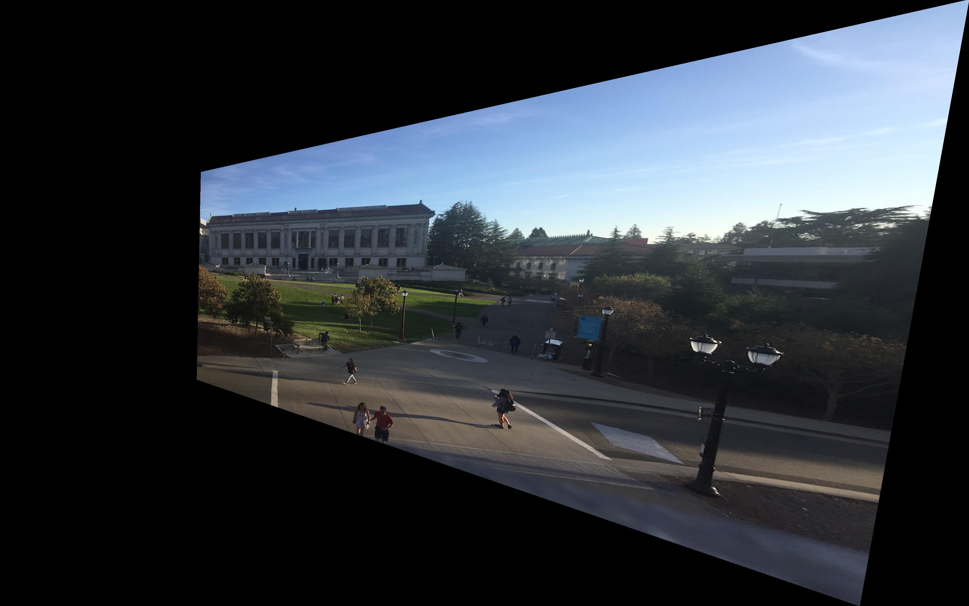
For image rectification, we identify the set of points we want transformed, and by taking the transformations of the four corner points, we know the range of points that our image will be transformed to. Knowing that, we use the inverse of the homograhpy matrix to perform inverse warping. Below is an example of image rectification.
Blending Images into a Mosaic
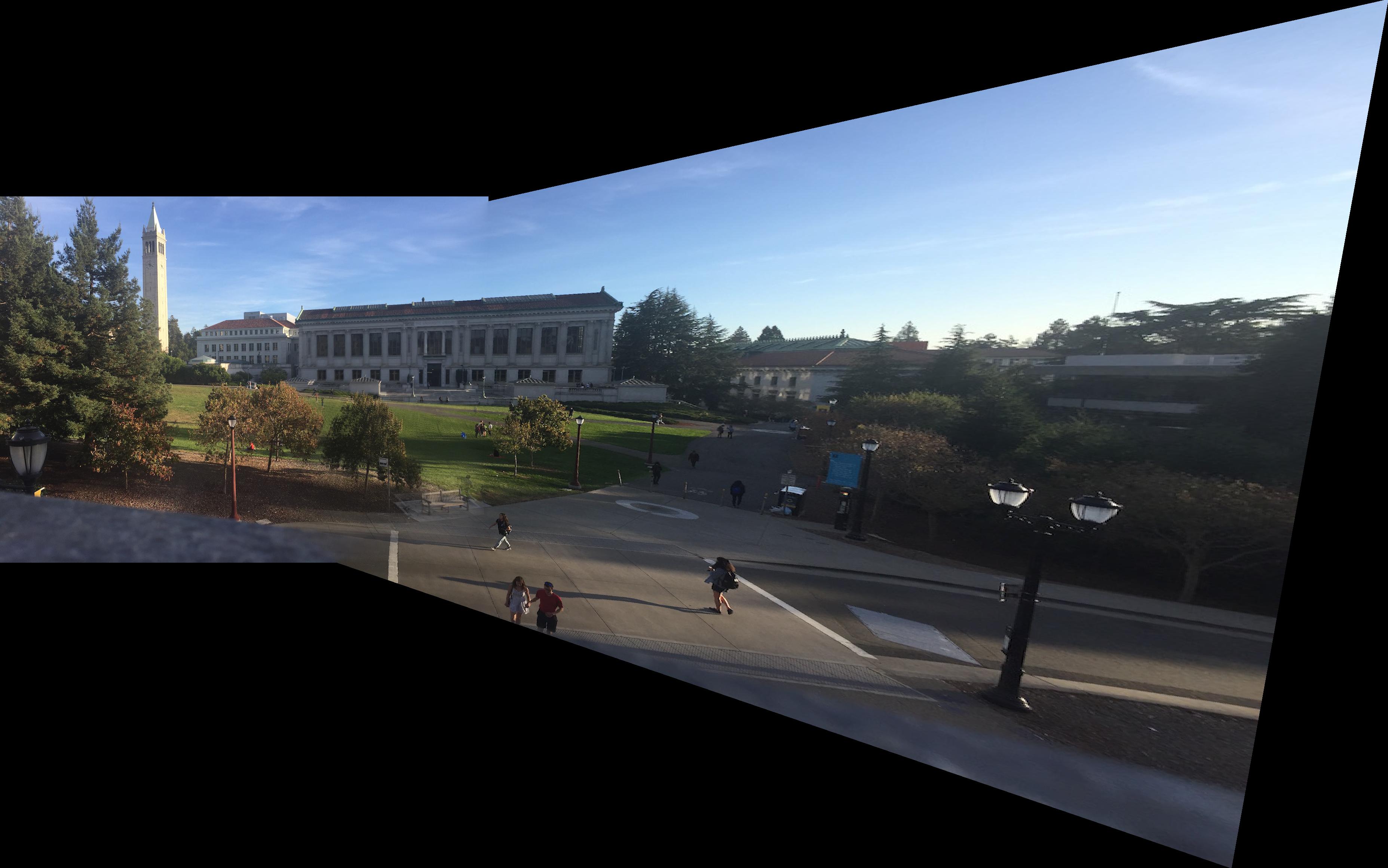
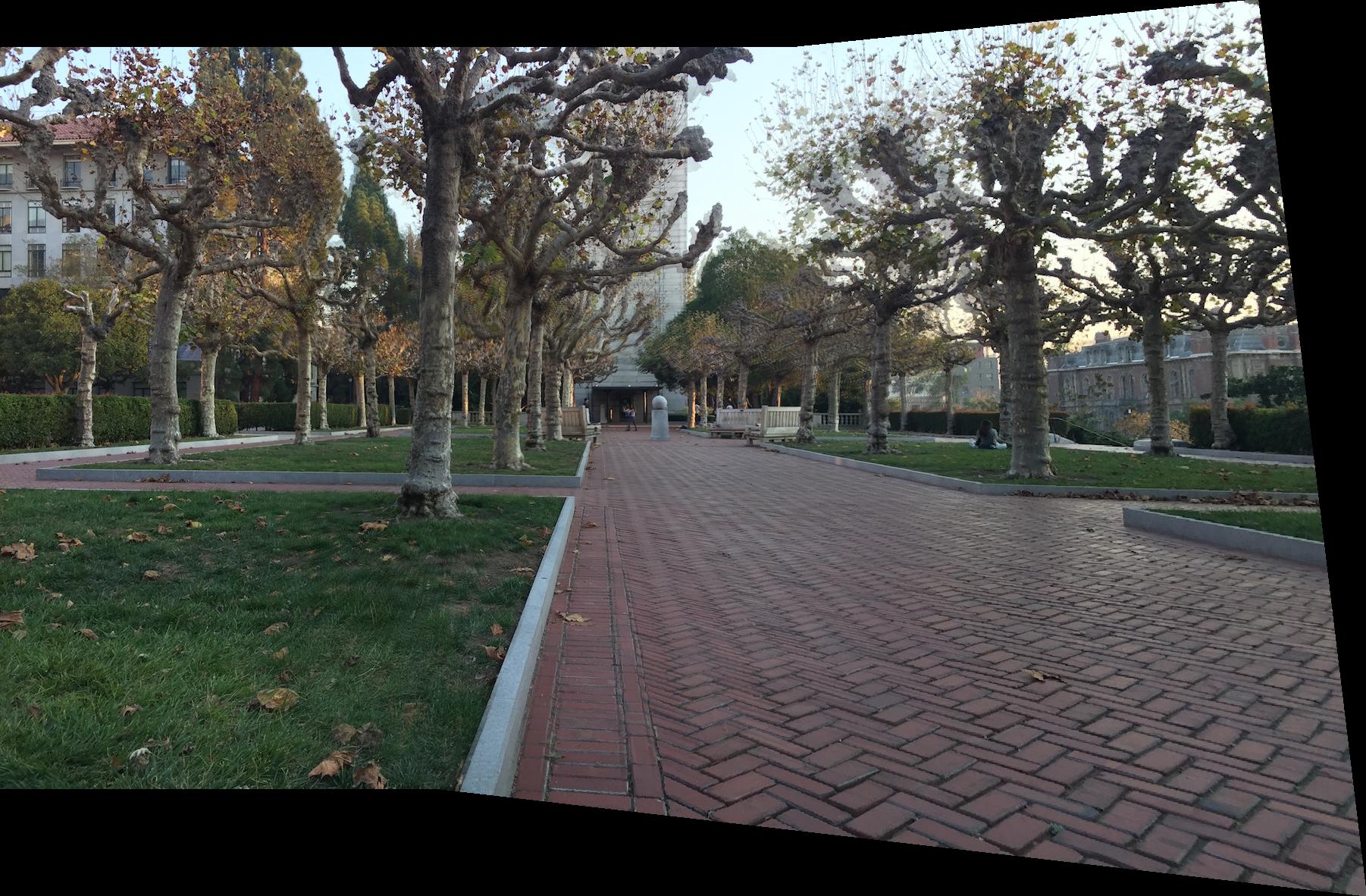
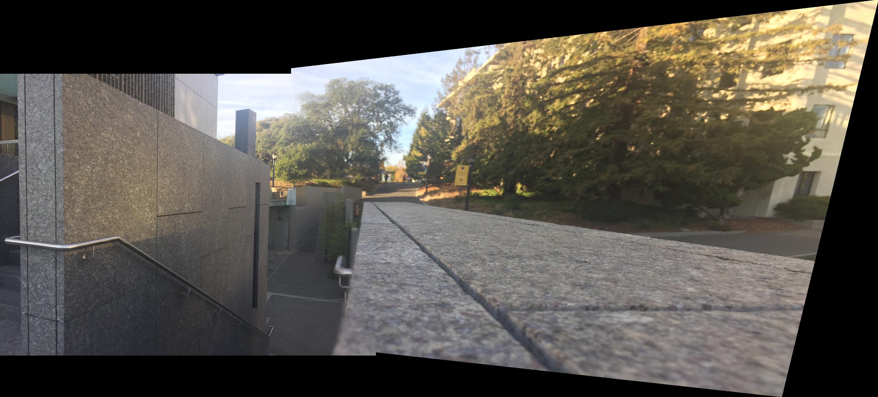
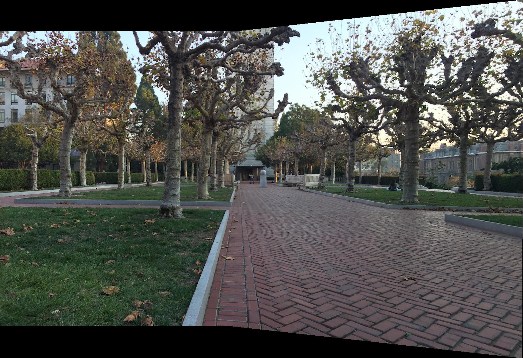
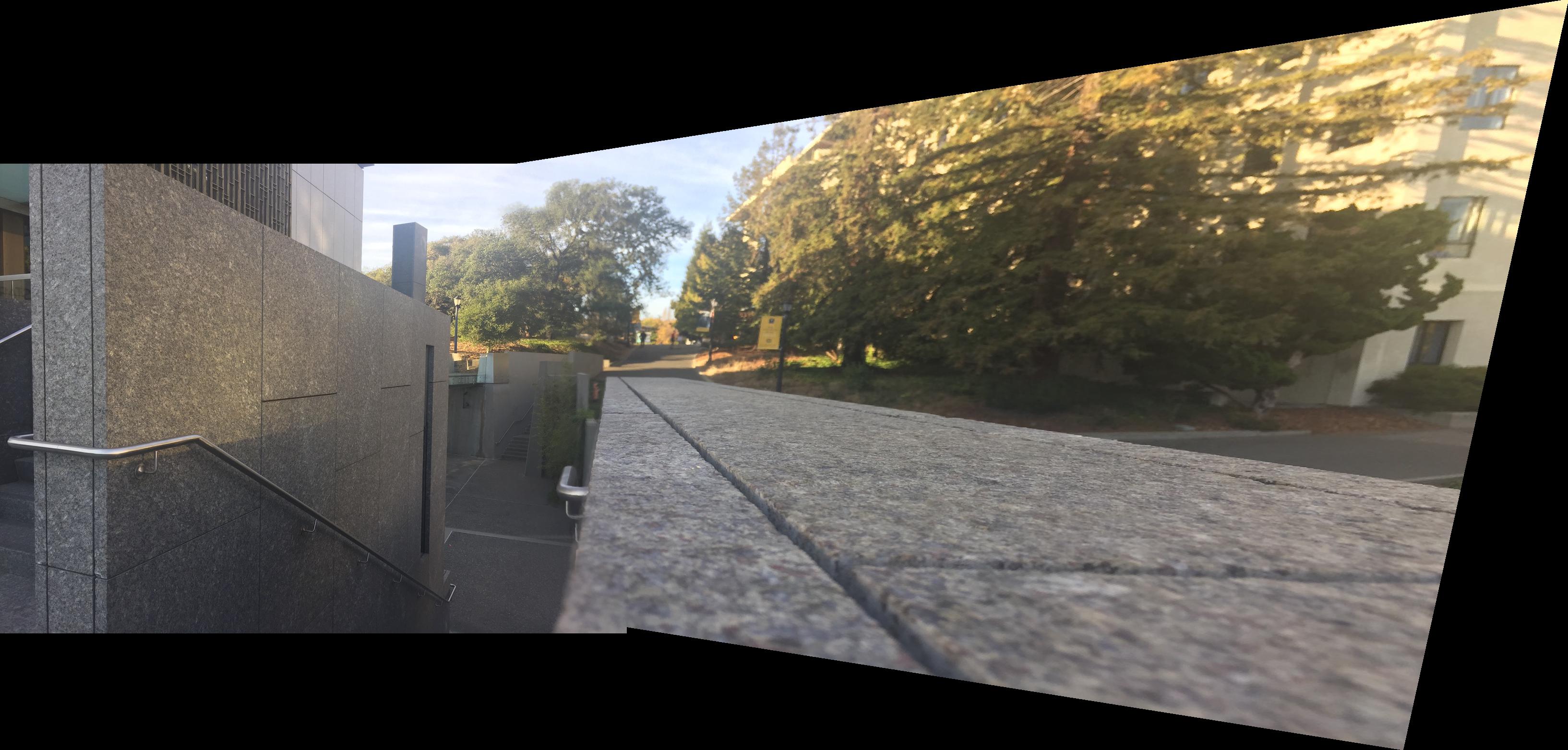
Using the previous parts, we combine them to form a mosaic of multiple images. To get rid of artificats that come from combining photos, we can blend them with weighted averaging by creating masks that have values depending on how close to each image's center the common point is and then blending using the masks (center weighting). We can also use laplacian pyramids on top of this as well.
What I've Learned
The most important thing I learned from this part of the project is that blending requires coming up with the right approach, which in this cases requires a 2d mask in order to get rid of both horizontal and vertical artifacts. The coolest thing I learned from this part of the project is how homographies can be useful to get interesting views of a certain part of the image, such as floor tiling as presented in lecture.
Part B
Harris Interest Point Detector
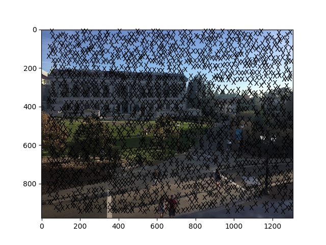
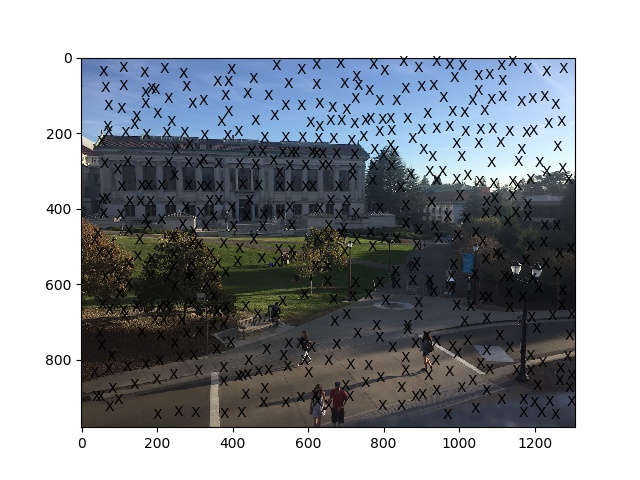
We use Harris Interest Point Detector to automatically find features/points in our image. It works by checking the gradient at each point of the image, and if it has a relatively large gradient for both the gradient with respect to x and with respect to y, then it is likely a corner. More specifically, the corner strength at a location is the determinant of the Harris matrix divided by the trace of the Harris matrix, where the Harris matrix is smoothed outer product of the gradients at the position. This process can be enhanced by doing it at multiple levels of a Gaussian pyramid. Below are images overlayed with the Harris corners detected.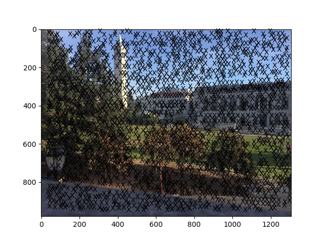
Adaptive Non-Maximal Suppression
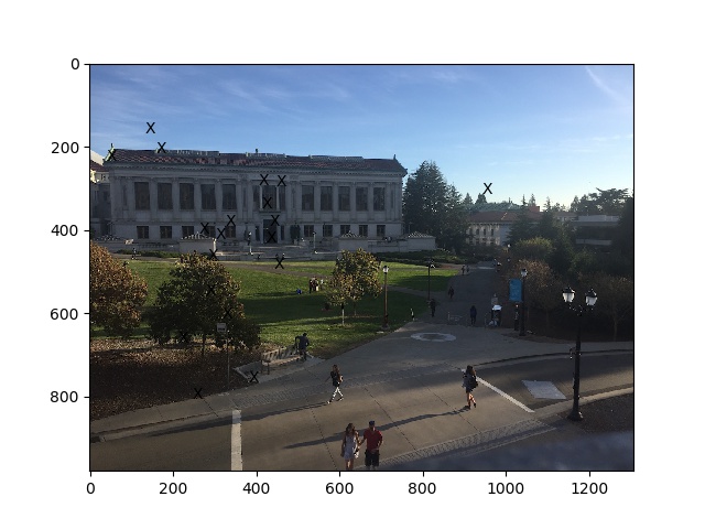
To reduce the number of Harris corners, we run adaptive non-maximal suppression. This algorithm finds the n points that have the largest minimal suppression radius, which evenly distributes the points selected spatially. The minimal suppression radius is defined as the minimal 2-norm between a point and another point (both in our list of Harris corners), such that the corner strength of our point is less than the corner strength of the other point multiplied by a robustness constant (we use c=0.9). Notice that the point with strongest corner strength might not be surpressed, and would thus have a minimal suppression radius of infinity. Below are images overlayed with the Harris corners remaining after ANMS.
Feature Descriptor Extraction and Feature Matching
For each point we have left, we do feature description extraction by taking a 40x40 patch around the point and then going to a lower frequency by blurring and subsampling down to a 8x8 patch. It is important to then normalize the patch to 0 mean and 1 standard deviation to make the features invariant to intensity. Using these features, we then try to find matches with the features in the image we are trying to stitch it with. We do so by finding the SSD between every pair of patches from different images. Theoretically, the best match would be its nearest neighbor, which minimizes the SSD. But it is possible to have incorrect matches, so we have a threshold (we use 0.5 here) that the ratio of the 1-NN over the 2-NN should be below, which gives better results because for a correct match, the SSD with the 1-NN should be a lot smaller than that of the 2-NN. Below is a pair of images overlayed with the remaining feature pairs after thresholding.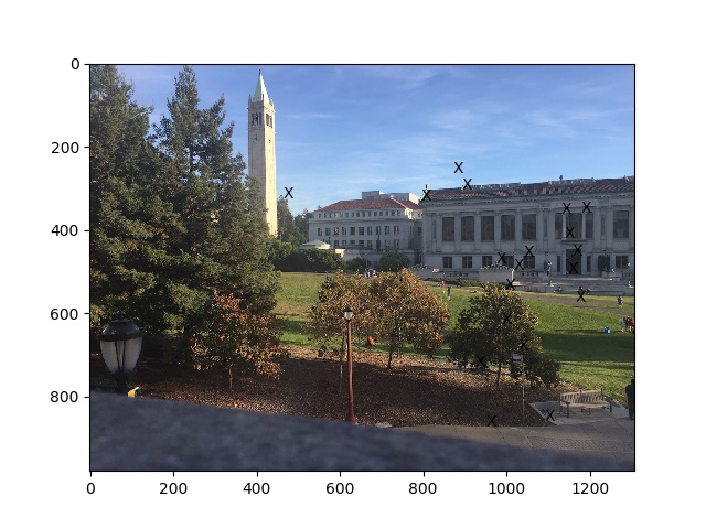
RANSAC
To compute homography matrices, we use 4-point RANSAC. This procedure takes four pairs of random points from the list of matched points from the previous step and computes an exact homography, before checking how many of all the matched points are within a certain epsilon of the transformation by homography, calling them inliers. After running this for a deterministic number of times, we pick the iteration that had the most inliers, and compute an exact homography the corresponding inliers. Below are the results of using said H to blend images, compared to using manually defined correspondences from part A.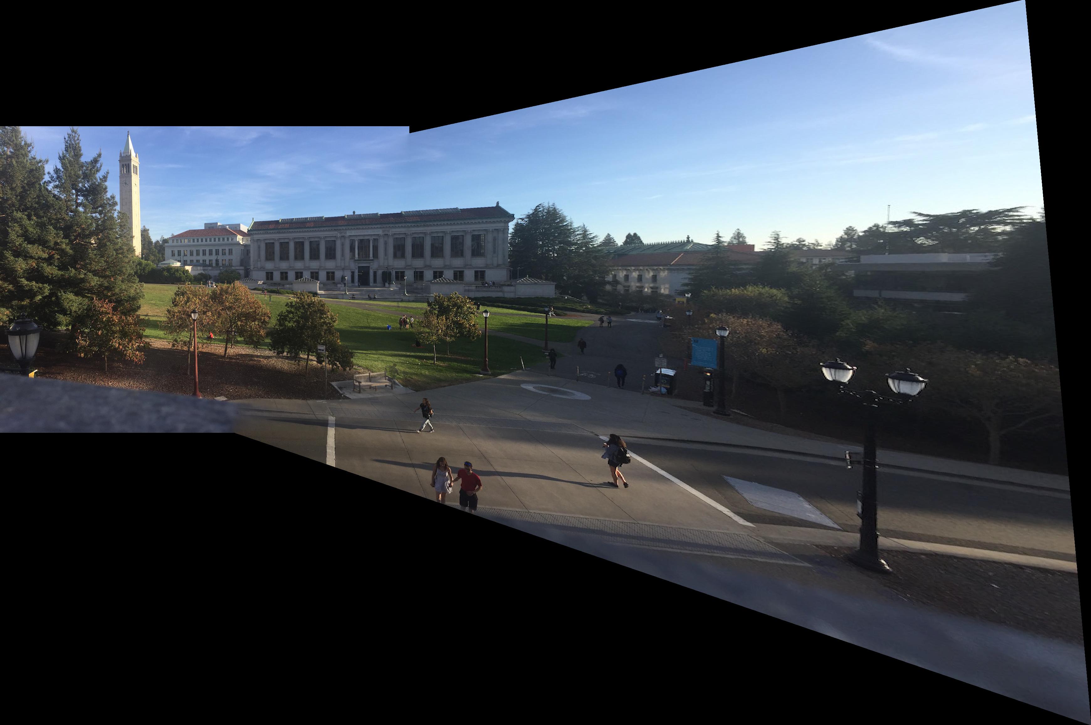
What I've Learned
In this part of the project, the coolest thing I learned is how in this instance algorithms were layered on top of each other to improve results. ANMS and Multi-Scale Oriented Patches both build on top of Harris corners to improve its initial results to find good features, which are then matched to automatically stitch together a panorama.