Programming Project #6: Image Warping and Mosaicing
This project focuses on warping images in order to blend them together in order to form a mosaic. I've always been curious
about how the iPhone constructs its panorama photos, so I found this project very interesting. I also found the math aspect of
this project rather challenging, since this was one of the first time we were working in the z-plane in addition to the x and y.
Image Warping
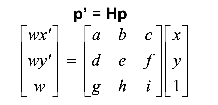 In this case, the transformation for warping an image is a homography. You can see on the right that the homography matrix
should transform a given point into its warped position. To solve for the variables in the homography matrix, I set up an equation
Ax = b where b held the coordinates that I was trying to warp my image into. I had some difficulty setting up the A matrix for
this equation, but eventually after some help from Piazza, managed to create a 3x3 homography matrix.
In this case, the transformation for warping an image is a homography. You can see on the right that the homography matrix
should transform a given point into its warped position. To solve for the variables in the homography matrix, I set up an equation
Ax = b where b held the coordinates that I was trying to warp my image into. I had some difficulty setting up the A matrix for
this equation, but eventually after some help from Piazza, managed to create a 3x3 homography matrix.
Image Rectification
After figuring out how to set up an equation to solve for a homography matrix, I inputted my corresponding points from an image. To
warp the image to be frontal-parallel, I chose objects in the images that were rectangular or square and used the corners as points.
I then clicked an approximation of the shape that the object should be if the image were to be frontal-parallel and entered these
as the parameters for my calculateH function.
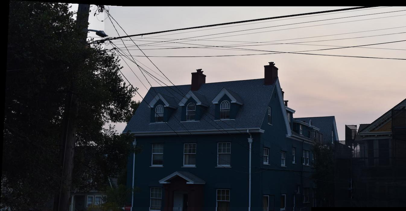
Once I got the homography matrix, I used inverse-warping to create the final image. This was similar to previous projects, with the main
difference being that after I got the x and y coordinates from taking the dot product of the initial points and H, I divided x and y
by the z value of the point in order to account for warping in the z-dimension. I additionally created a function to accomodate
for the larger dimensions resulting from the warped corners for the house image.
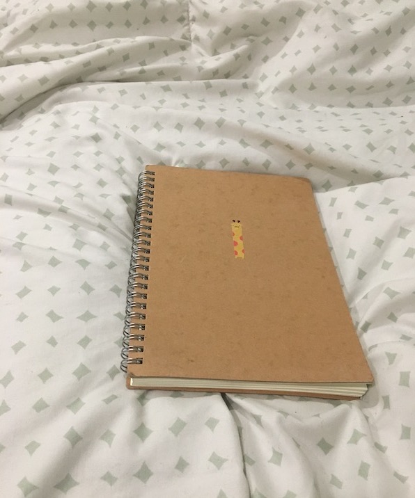
Notebook: Unwarped
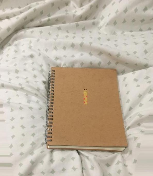
Notebook: Frontal-Parallel
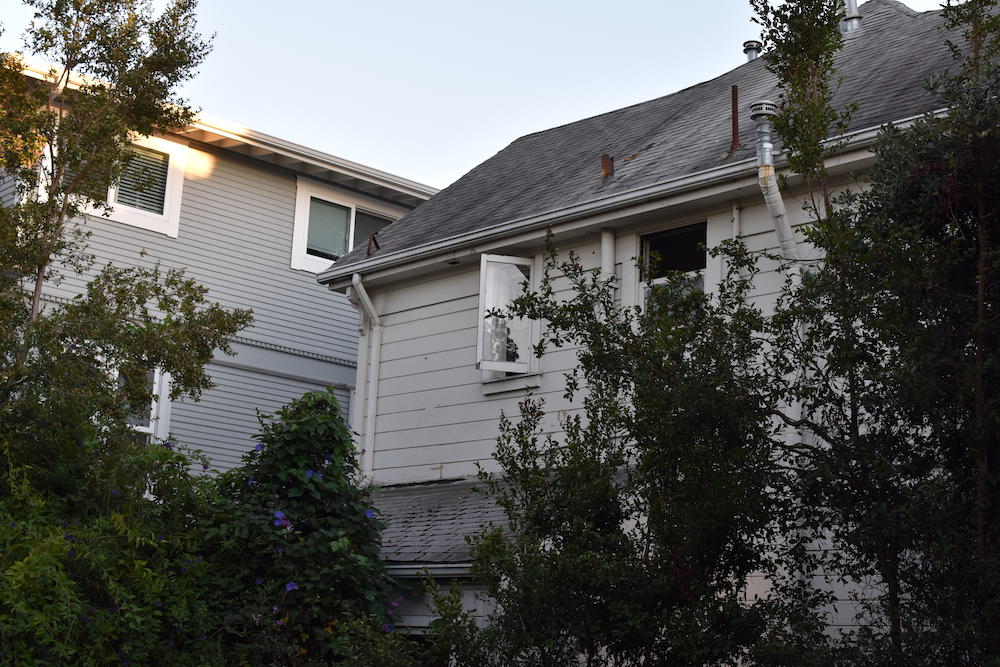
House: Unwarped
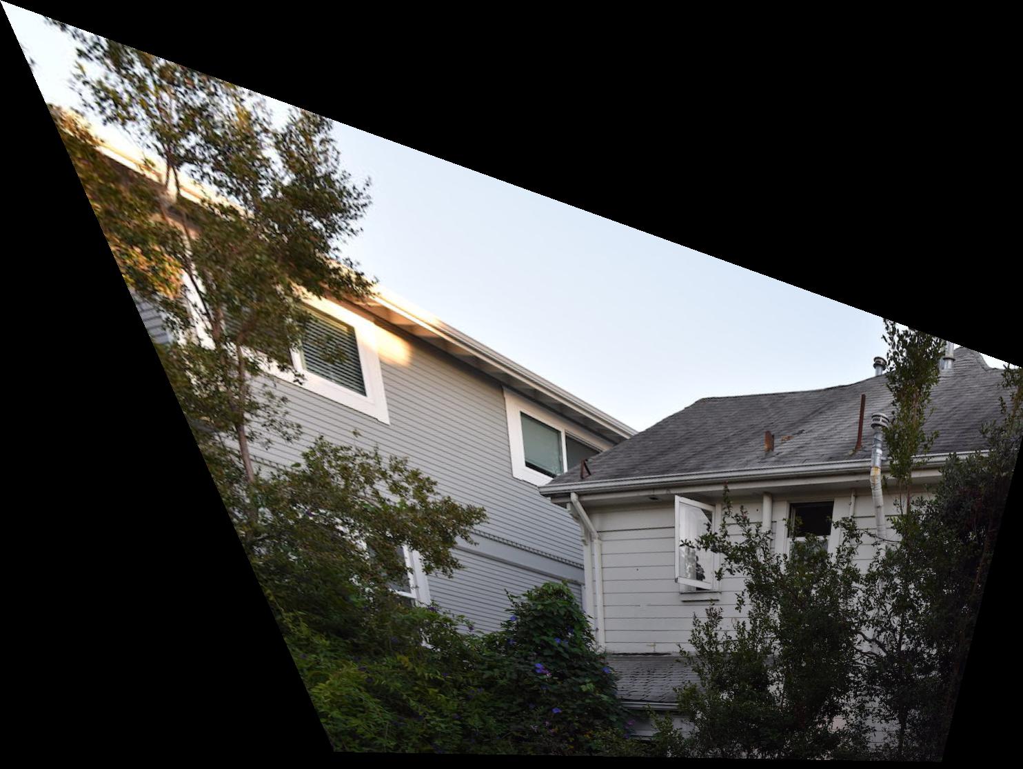
House: Frontal-Parallel
Blending Images into a Mosaic
To blend images together, rather than using a square or rectangle approximation like in the image rectification section,
I used corresponding points for overlapping features between the two images. Then I would warp one image into the perspective
of the other and then naively blended the two. When I used enough points, the naive blending worked rather well, but as you
can see, using 4 or 8 points had some misalignment. After realizing that 12 points provided the best results, I created three total mosaics as seen below.
4 input points
8 input points

12 input points
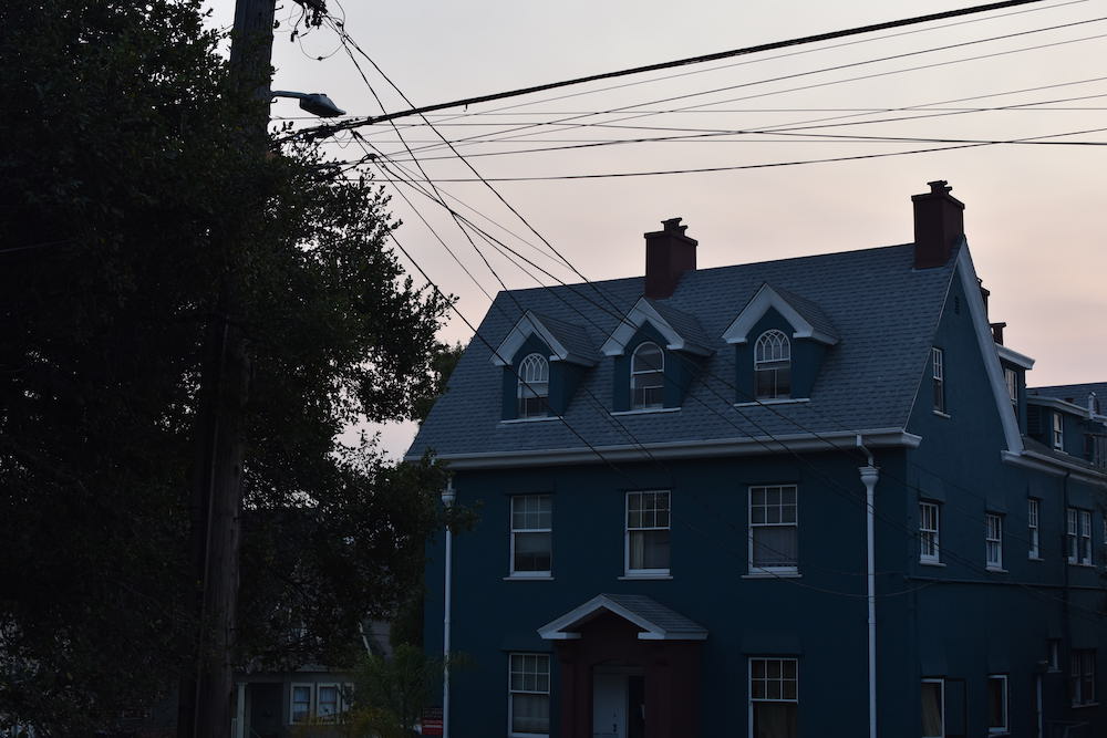
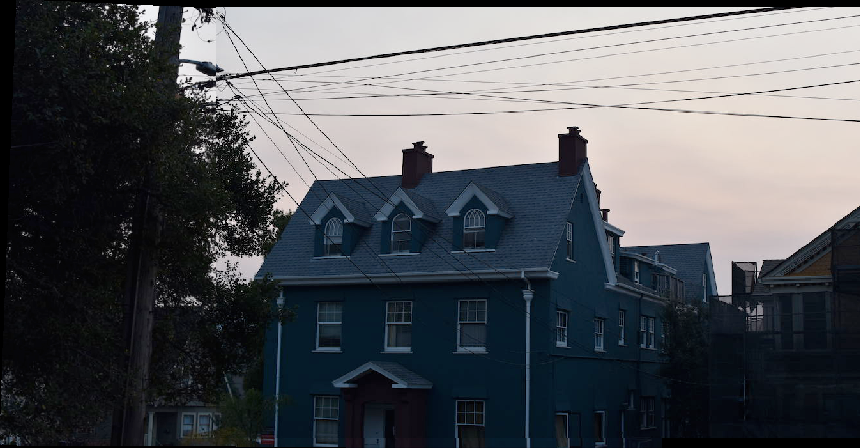
Image 1
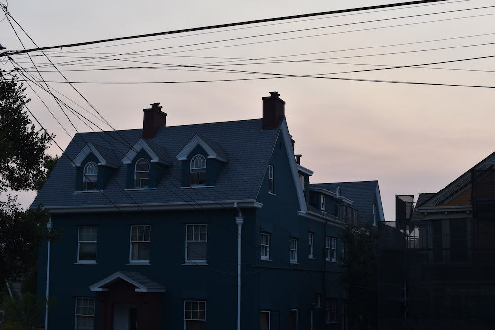
Image 2
Street View: Mosaic
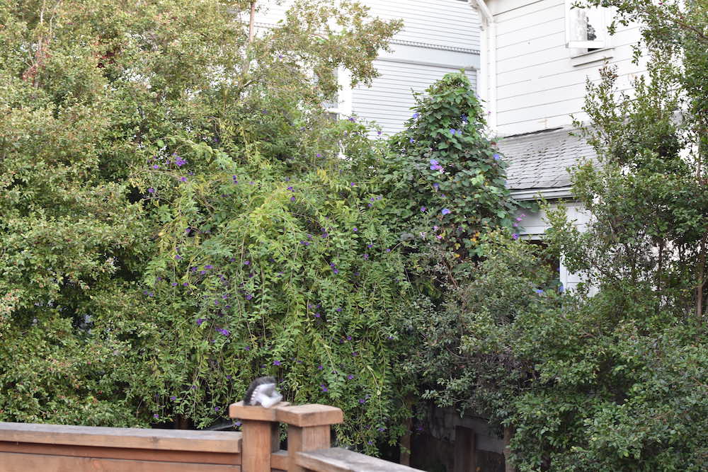
Image 1
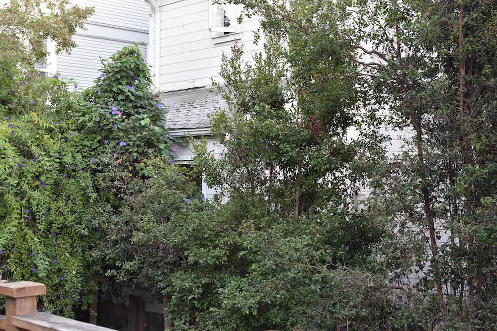
Image 2
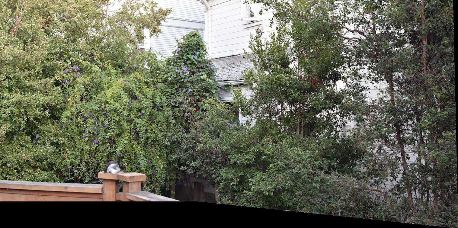
Vines: Mosaic
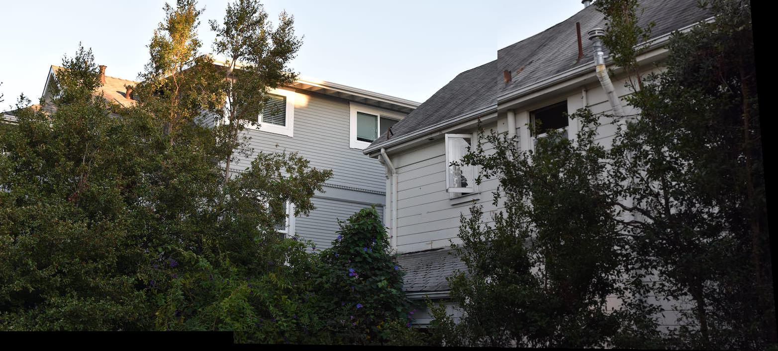
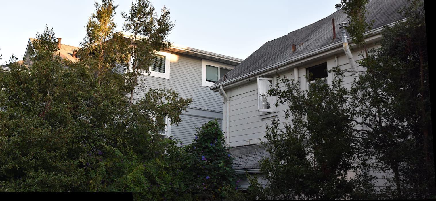
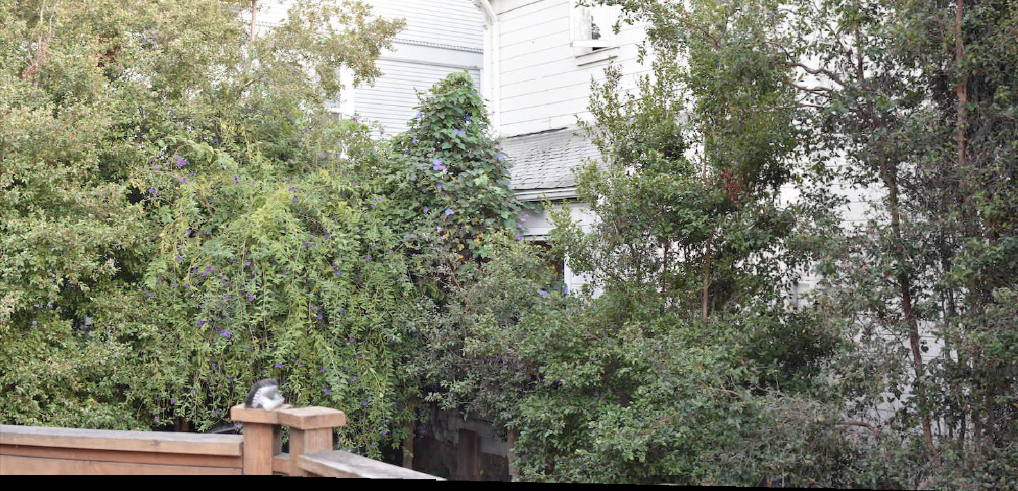
Image 1
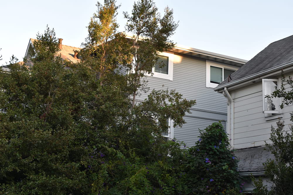
Image 2
House: Mosaic
Overall from this part of the project, I learned a lot more about what homographies are and how to solve for them.
It's different hearing about it conceptually in class and actually getting your hands dirty to code it yourself.
I realize that it's important to make sure the equations are set up correctly and that having more data points can
solve a lot of problems (as Professor Efros as said many times.) I honestly spent so much time trying to figure
out what was wrong with either my mosaic or warping function, only to realize that the mosaics were unsatisfactory
due to me using too little corresponding points as references. Despite the frustrations though, I genuinely
enjoyed this part of the assignment, since it answered some questions I've had for a while about stitching photos
together for panorama-style results.
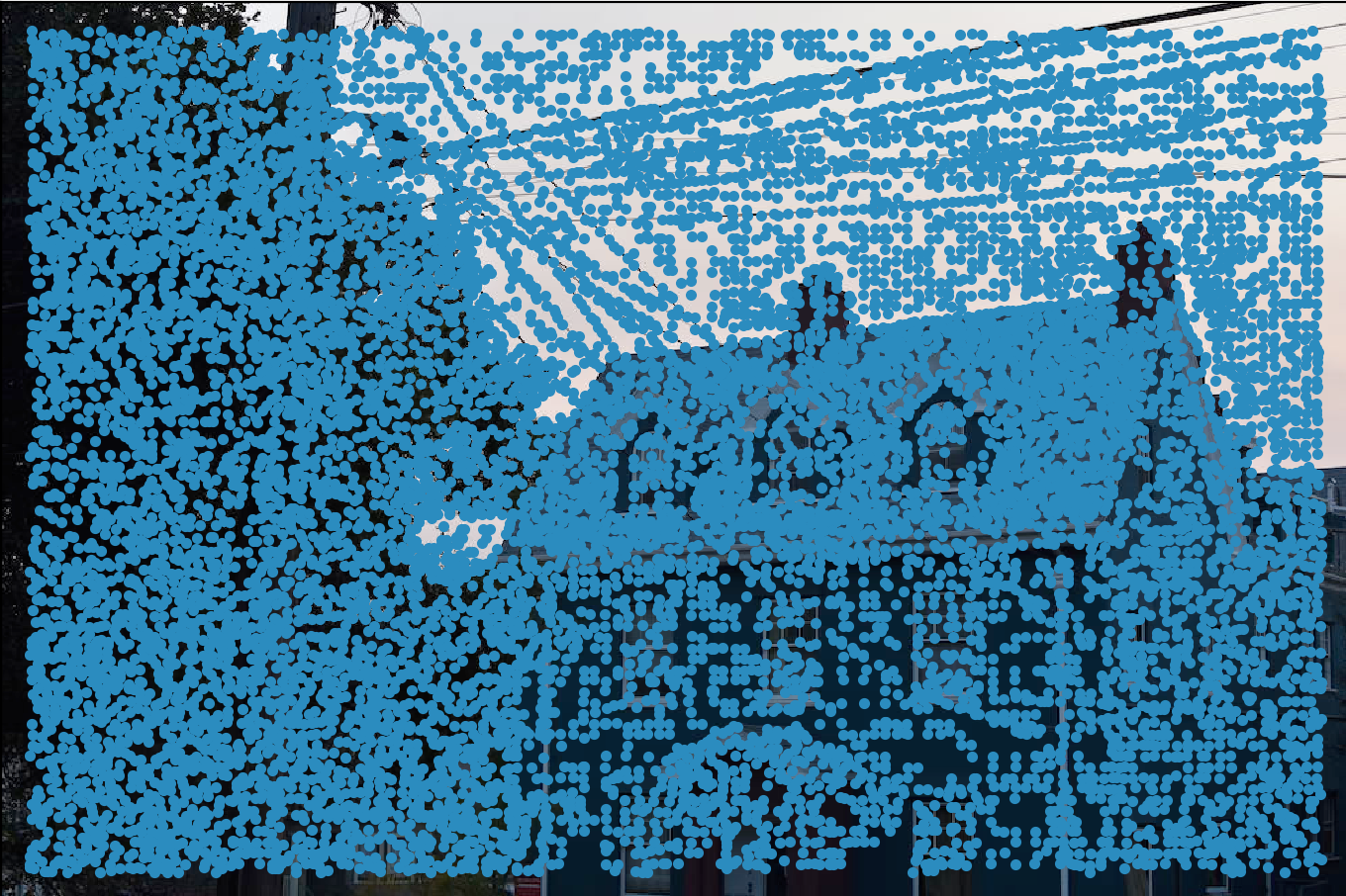
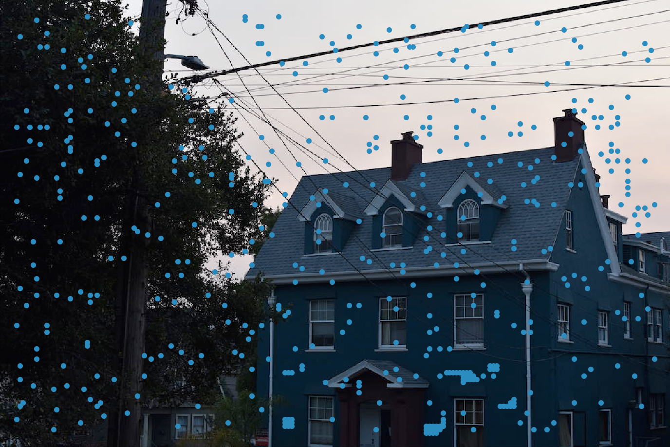
Harris Point Detector
This part of the project was fairly straightforward as the code for getting the Harris corners was already provided.
Below are the corners found through this method. As you can see, there are way too many points, but this will be taken
care of in the next steps. I've included images with both large and small dots for easier visibilty.
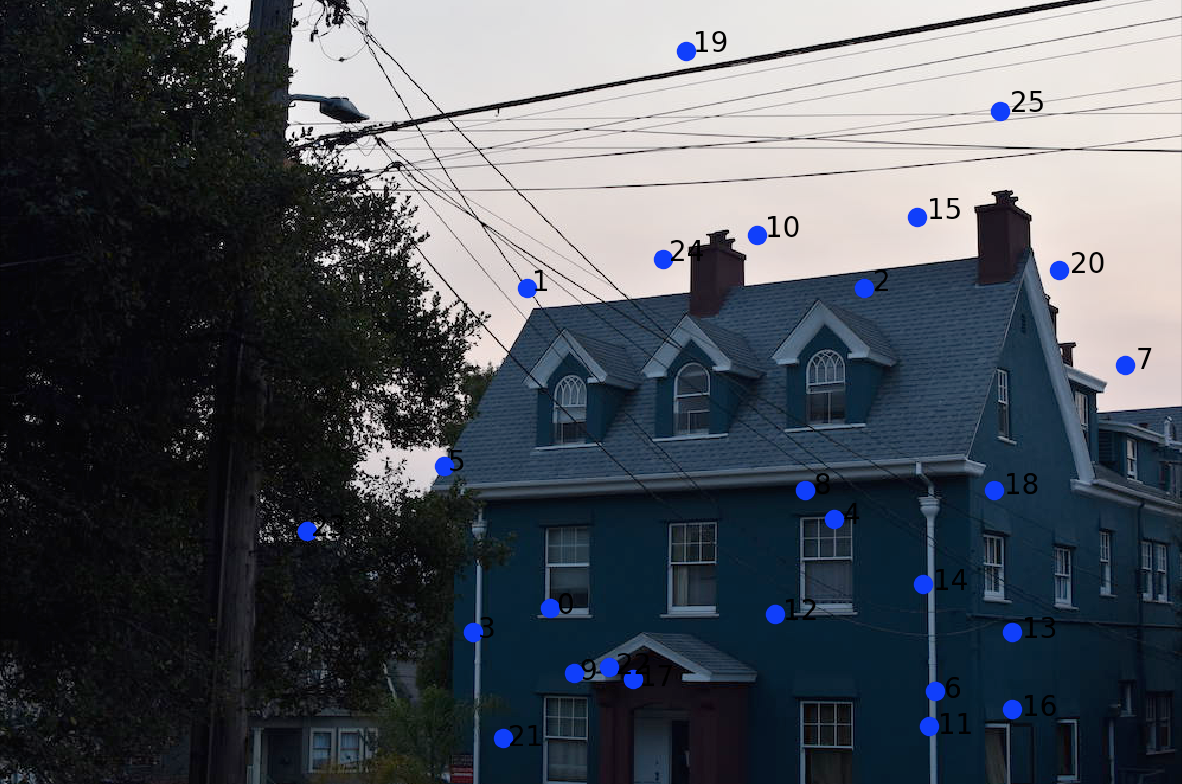
Adaptive Non-Maximal Suppression
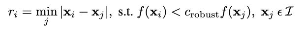 This part of the project took me a bit more time as understanding why the math worked involved reading through the section of
the paper several times. Essentially, the equation on the right means that we need to iterate through the points picked out from
the previous section's Harris point detector and filter out the best ones to use. We do this by finding the closest neighbor to
a point, making sure that the neighbor is at least 10% greater in strength that the point we are currently looking at. Then we keep track
of the minimum distance between each point and their respective closest neighbors and keep the 500 points that have the largest minimum distance.
This process ensures that the points chosen are spread out from each other, which might not be the case if we simply chose points that had the
highest strenghts.
This part of the project took me a bit more time as understanding why the math worked involved reading through the section of
the paper several times. Essentially, the equation on the right means that we need to iterate through the points picked out from
the previous section's Harris point detector and filter out the best ones to use. We do this by finding the closest neighbor to
a point, making sure that the neighbor is at least 10% greater in strength that the point we are currently looking at. Then we keep track
of the minimum distance between each point and their respective closest neighbors and keep the 500 points that have the largest minimum distance.
This process ensures that the points chosen are spread out from each other, which might not be the case if we simply chose points that had the
highest strenghts.
Remaining points after ANMS
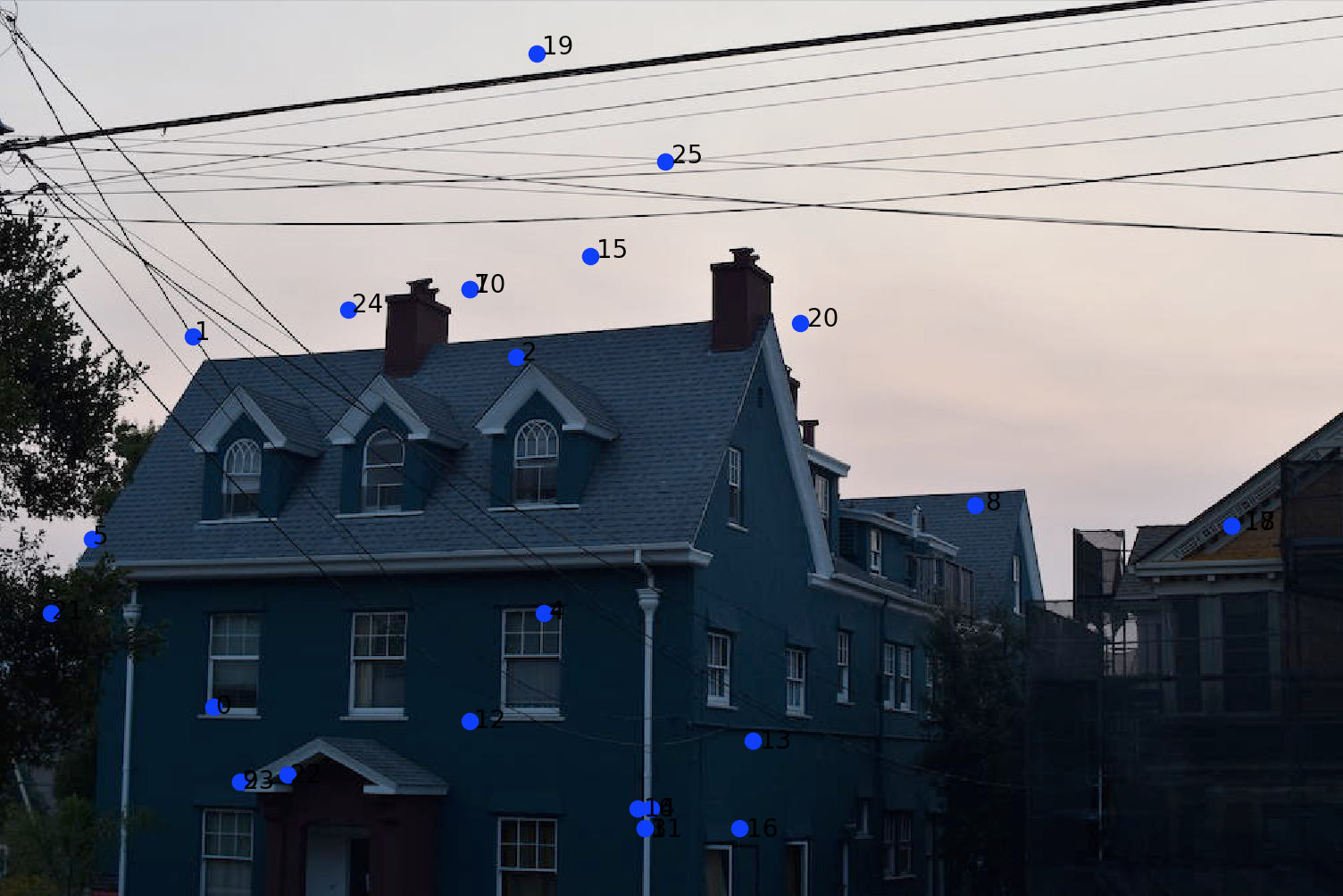
Feature Descriptors and Feature Matching
Now for the points we have remaining after ANMS, we wish to construct 8x8 patches that serve as feature descriptors. We sample
this patch from a larger 41x41 window around the point in order to have a more blurred descriptor. After downsizing this larger
window to the desired 8x8 patch size, I normalized the patch so that the mean is at 0 and the standard deviation is 1.
Below is an example of a feature patch from the nineteenth point.
After generating points and respective feature descriptors for the two images we'd like to combine, we need to pair the features
with their best match. I employed the provided dist2 function from the source code as a metric. The patch that has the lowest dist2
value for another match is the match's best neighbor, while the next lowest dist2 value is its second best neighbor. We use the ratio
of the best neighbor to the second best neighbor (1NN/2NN) as a threshold for determining whether this matching is sufficient to keep. At the
end this results in corresponding points between the two images, which in part 6A of the project had to be manually selected.
RANSAC
The next step after obtaining corresponding points is to generate the homography. To provide a better estimate, we first
select four corresponding points at random and generate a homography. Then we use this homography and test it with all of our
corresponding points, keeping track of how many inliers there are. After repeating
this many times, we choose the largest set of inliers and recalculate the homography on these points to get the final homography.
We then proceed as in part A of the project and use this homography to generate a mosaic.
Street view with manual stitching
Street view with automatic stitching
Vines view with manual stitching
Vines view with automatic stitching
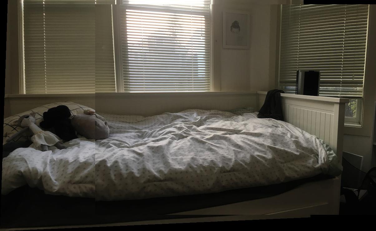
Bed view with manual stitching
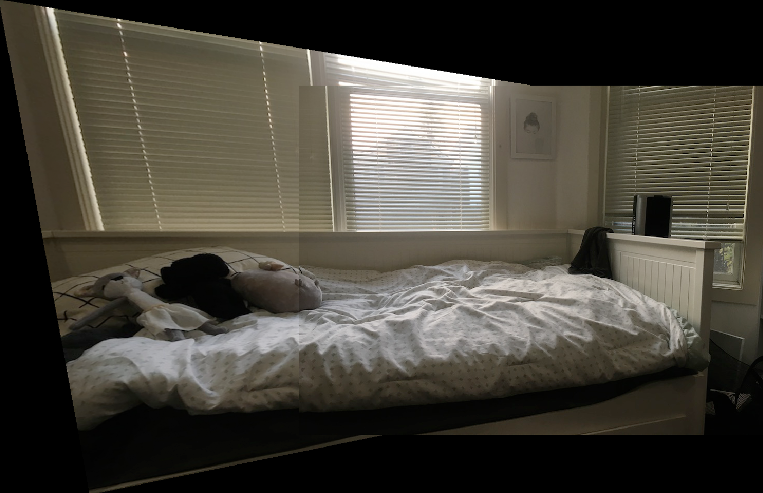
Bed view with automatic stitching
Overall from this project, I learned so much regarding the math for automatically stitching photos together.
It was interesting to see the different metrics used to judge the feature matching and filtering out of Harris
points. I struggled a bit with understanding how the math behind the procedures worked, but once I did, the coding
aspect was not too bad. There were some images that worked better than others due to the slight discrepancies
in color or rotation when I took the photos. This is largely due to my own fault when taking photos, not the algorithm.