Overview

In this project, we calculated the homographies, or image transitions, between sets of points, and used the homography to rectify images taken at different angles. We also used the homography between two sets of corresponding points to stitch two photos of different parts of a scene together into a larger photo mosaic. In the next part, we investigated automatic feature matching in order to compute homographies without manual point input. This involved finding harris corners, limiting the number of considered corners using ANMS, finding feature descriptors for each corner, and matching the features. Then we used RANSAC to evaluate the feature matches and remove the outliers before calculating the homography and warping the images together.

Section I: Manual Photo Stitching

Part 1: Shoot Pictures

For this assignment, it was important to take the images so that they were all rotated around the camera and not translated at all. This helps ensure that the homography is able to capture the transformation of the image between locations. Since I was using my phone's camera, I didn't have much control over my camera's settings, but I made sure not to deliberately change any of them.

Part 2: Recover Homographies

In order to compute Homographies, I took two sets of points, and used the quadratic relation between them to create the matrix below.

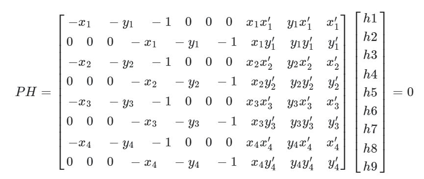
Part 3: Warp the Images

Once the homographies are calculated, I warped the image by finding all the locations in the original image that correspond to the pixels in the new image, and then pulling those pixels from the original image. I found the locations of these pixels using the inverse homography matrix. This essentially produces an image which is a free deformed version of the original.

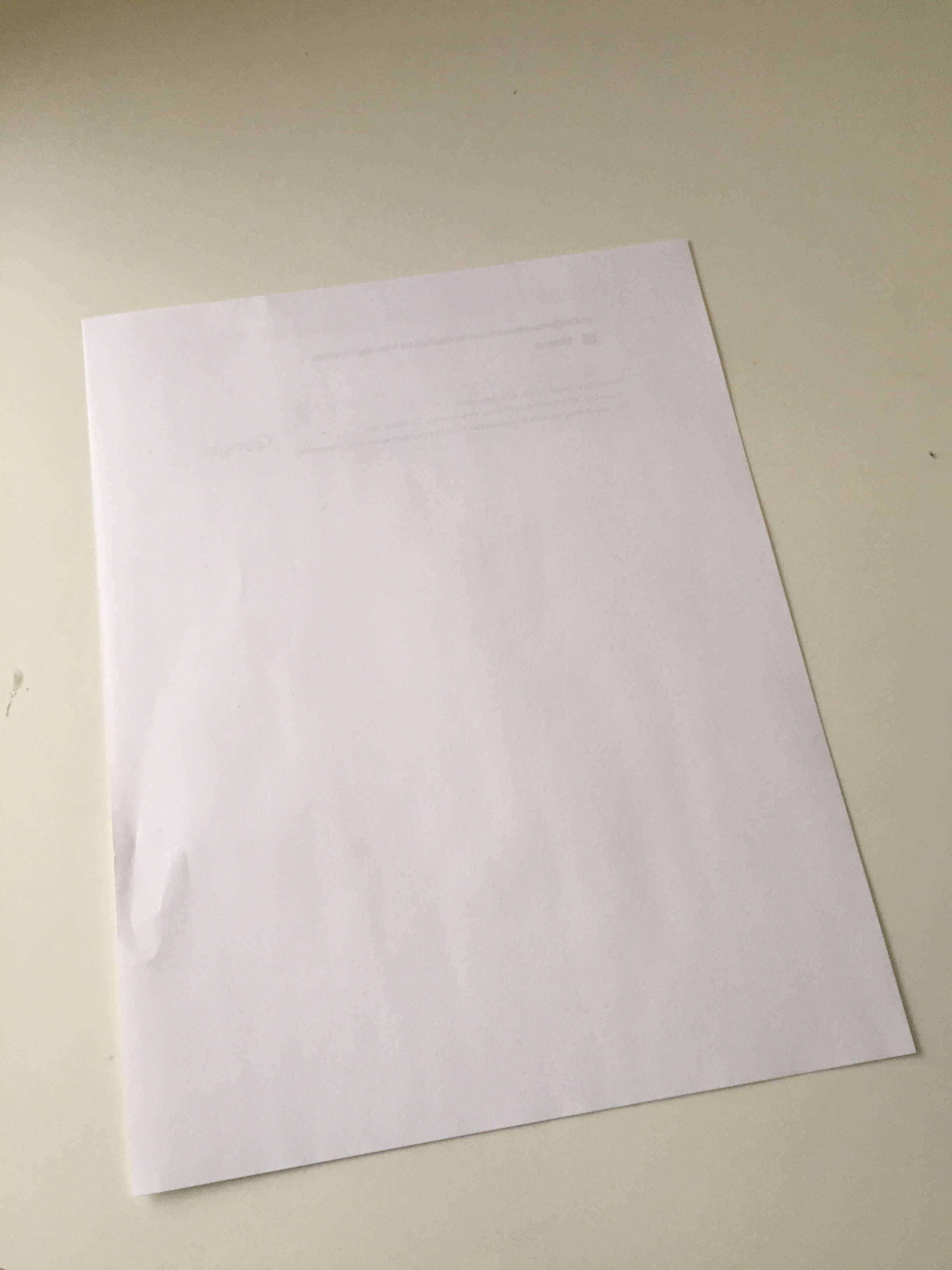
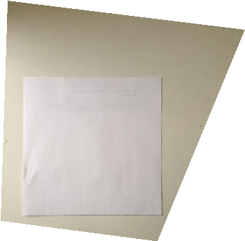
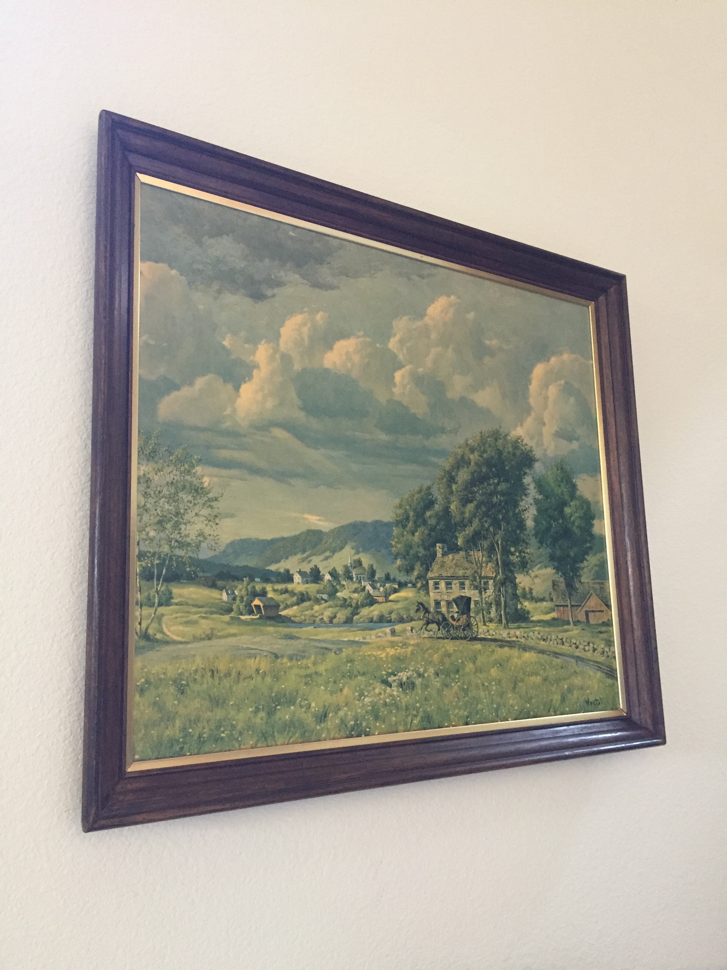
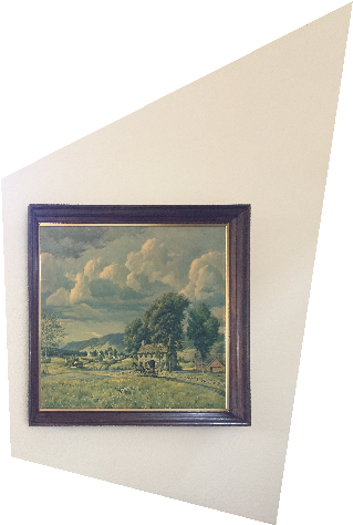
Part 4: Image Rectification

Warping an image of a rectangular object to a set of points that describes a rectangle will cause the object to appear rectangular as it should. Some results are shown below.

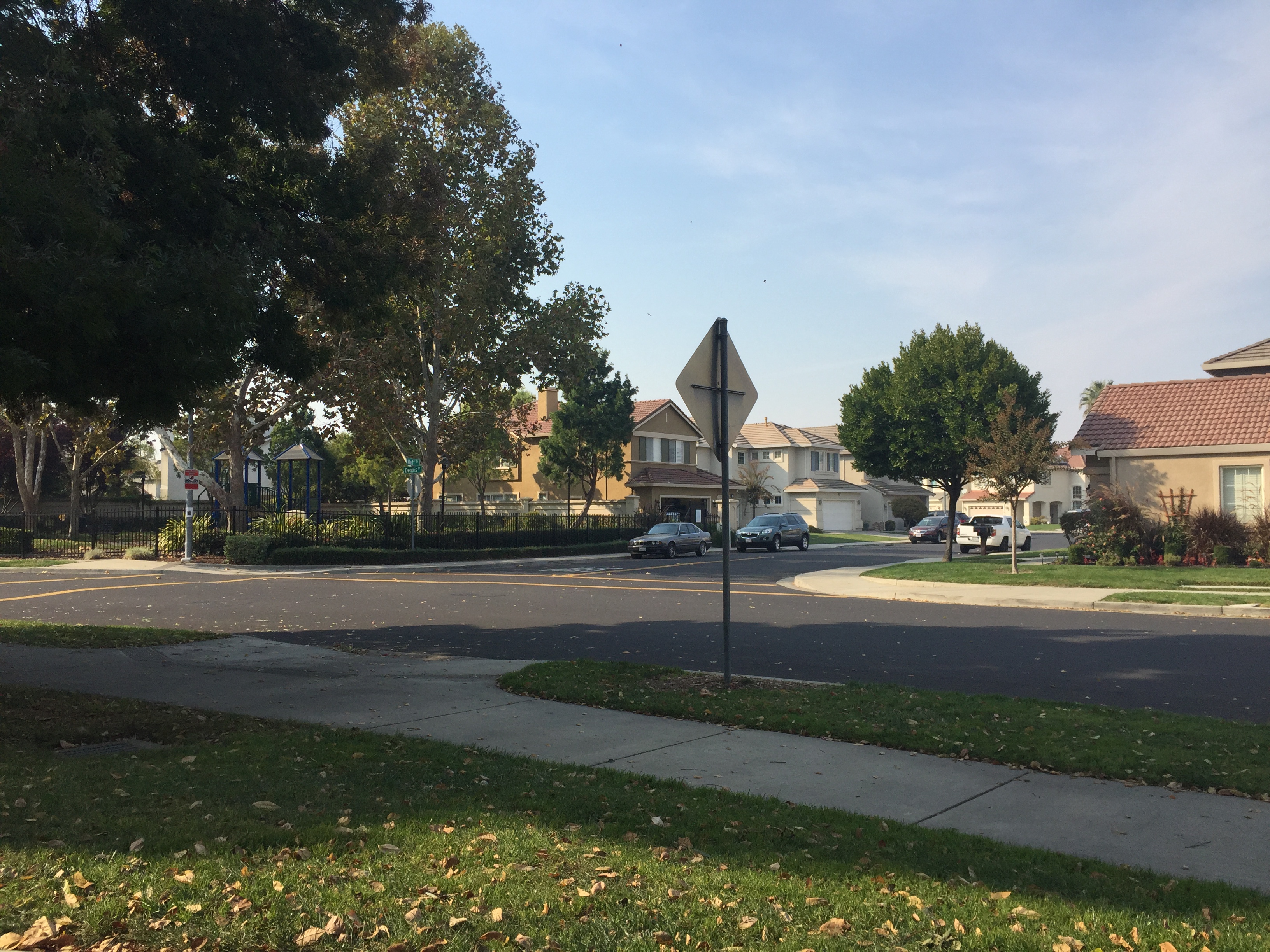
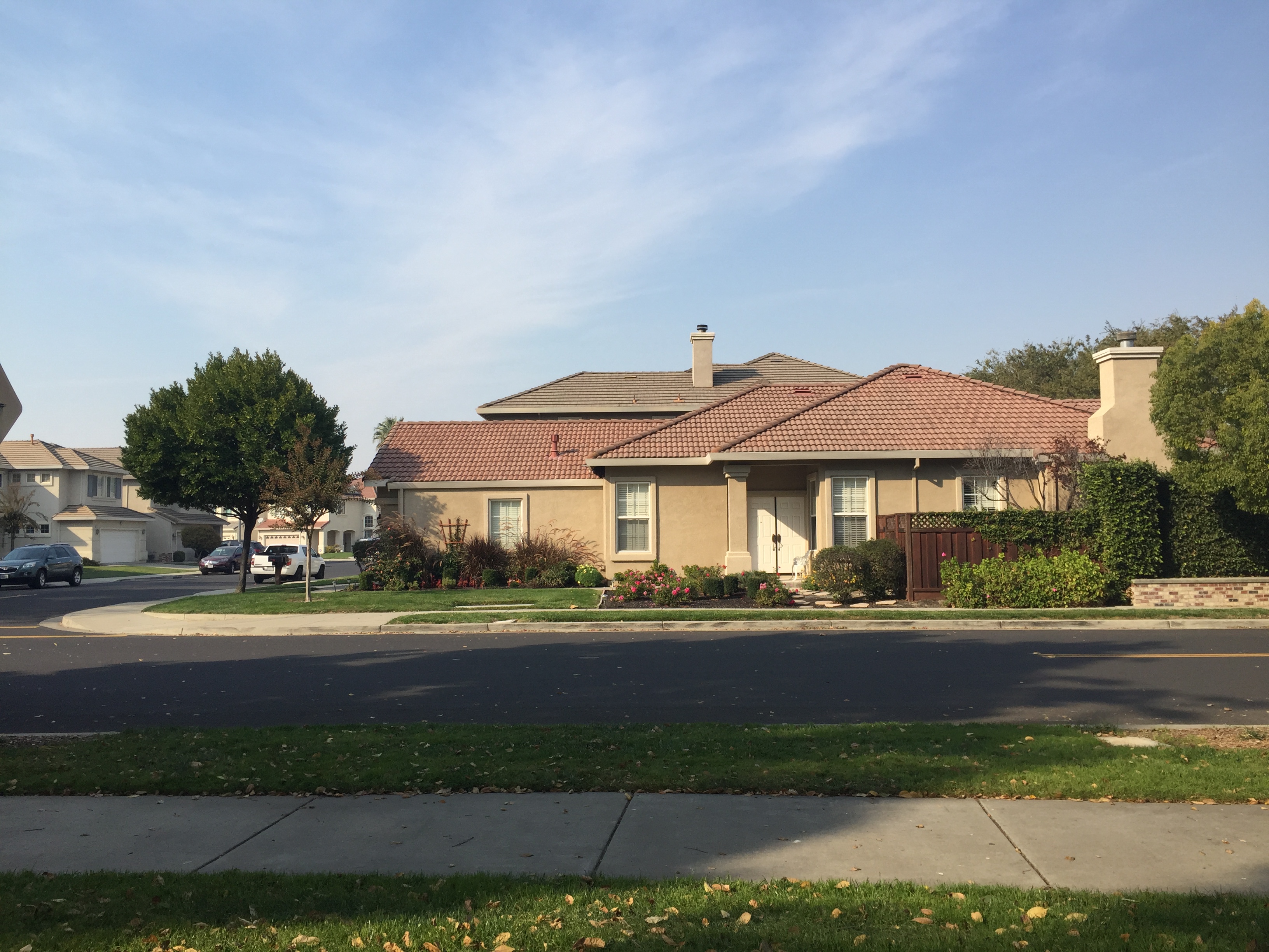
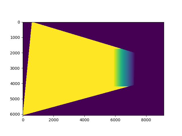
Part 5: Blend Mosaic

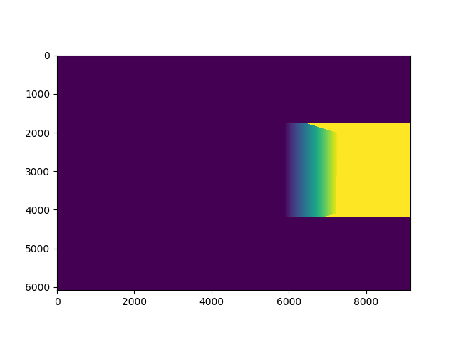
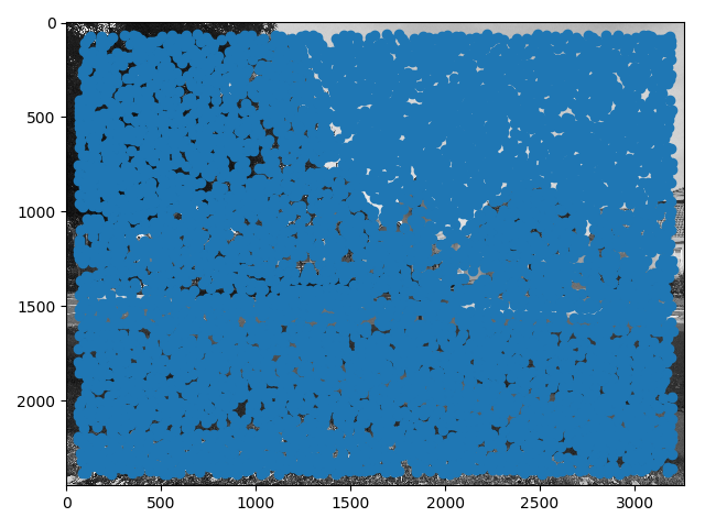
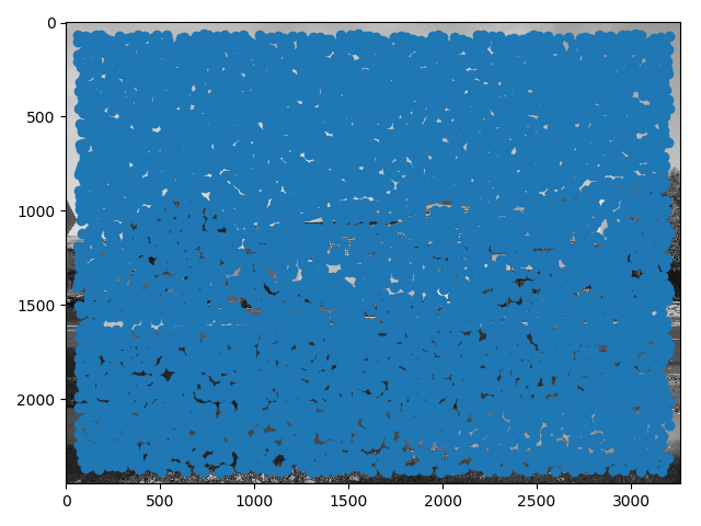
For this part, I warped one image into another using the homographies calculated from the previous steps, and using manually chosen pairs of points in both images. I then blended the two images together using a horizontal gradient mask. Below are the warps visualized as gradient masks, and the results.

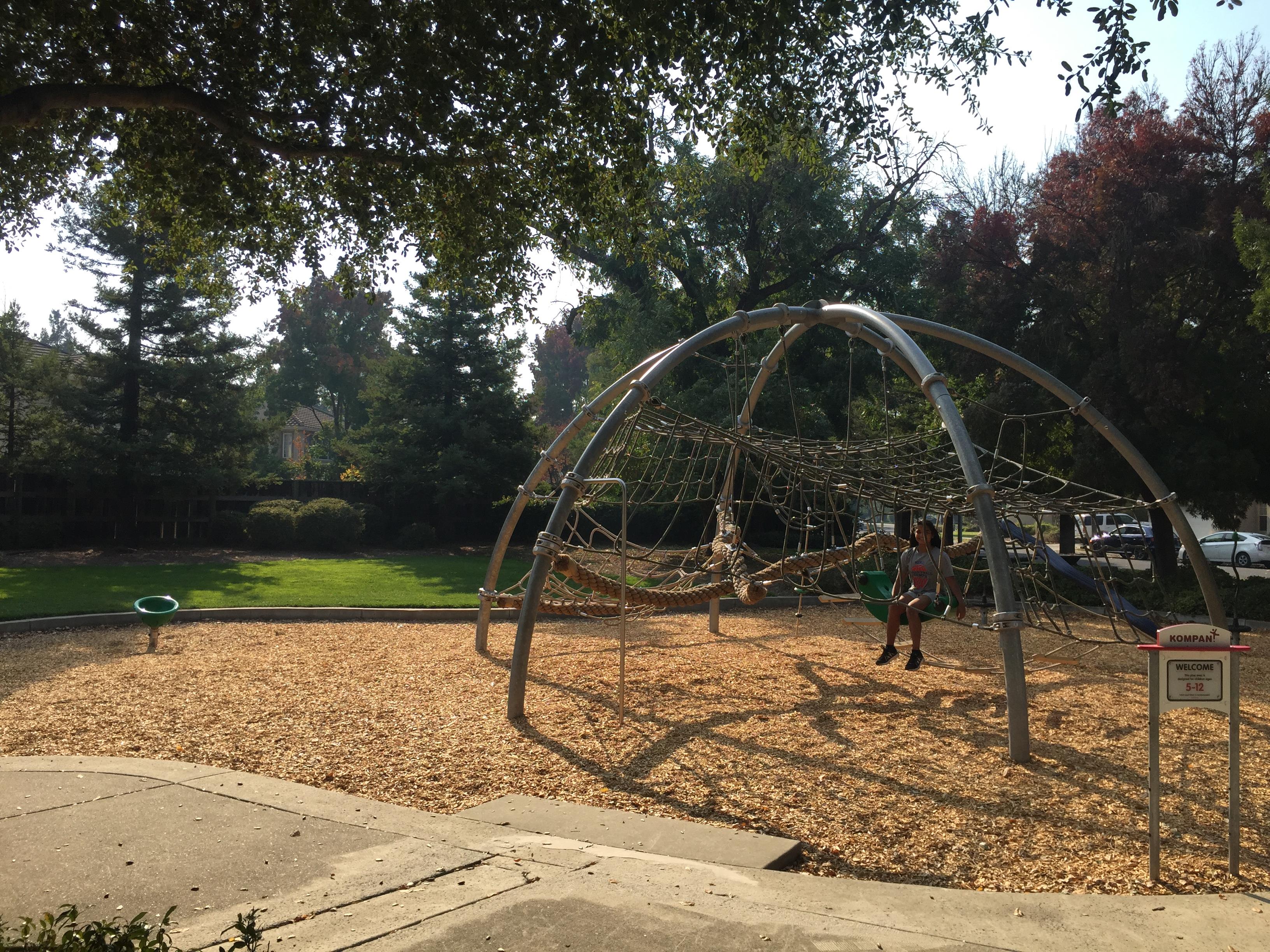
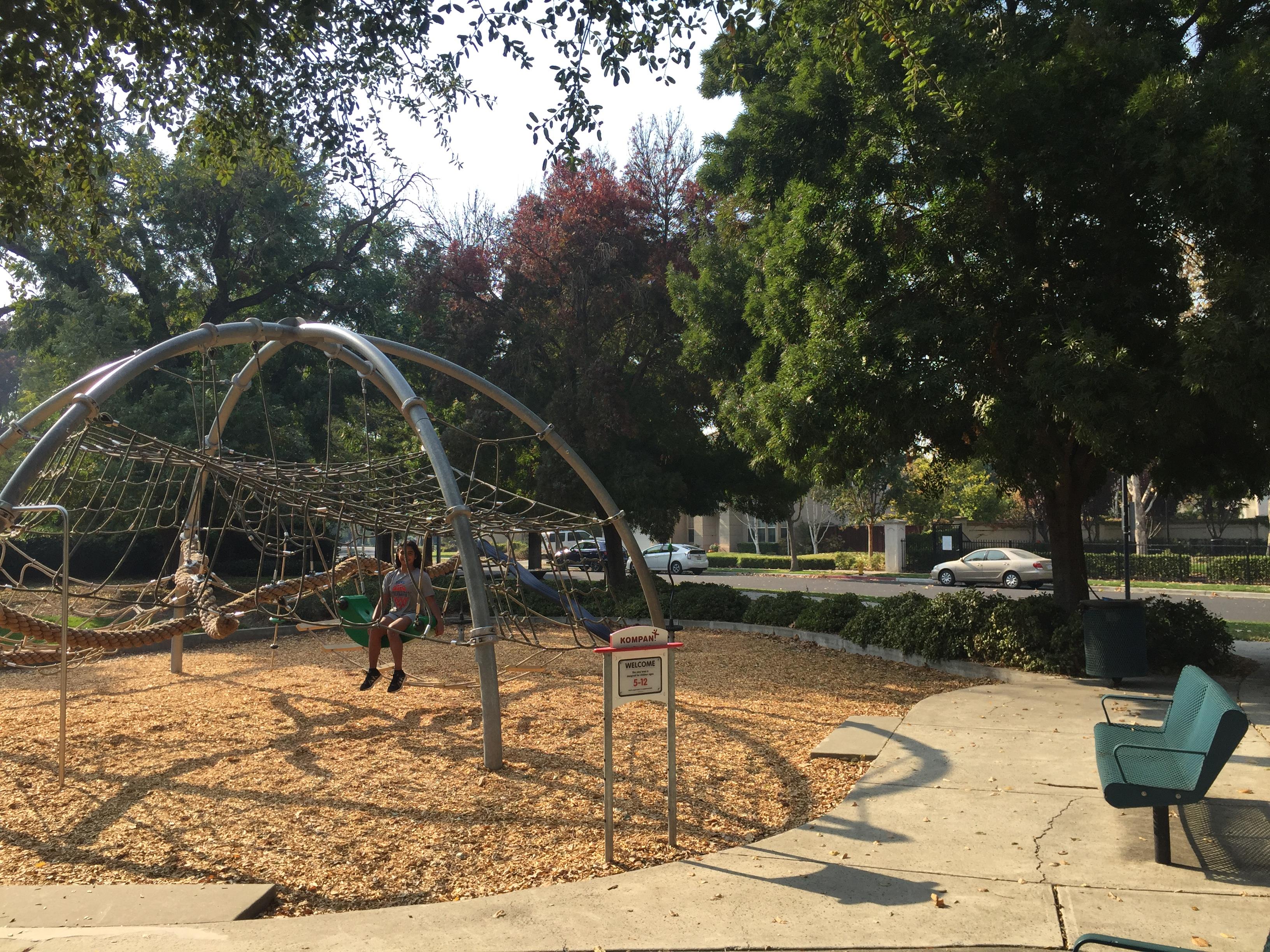
Manual point selection worked pretty well for the most part, it was just time consuming. One interesting thing to note is that the Playground image is a little blurry: this is because there was a wind blowing at the time and the trees in the background were moving because of it. The girl in the playground (my sister) was also moving a bit, but these effects are somewhat mitigated by the fact that I took these images using the handlebars of my scooter as a makeshift tripod, so I was able to take pictures quickly with minimal vertical translation.

Section II: Automatic Photo Stitching

Although manually choosing correspondence points is viable with only a few images, it's quite time-consuming to do for multiple images. To solve this problem, we investigated automatic feature matching.

Part 1: Harris Corners

In order to find features, we first need to find interest points, which can be thought of as potential features. To do this, I used the given code to calculate Harris Corners, which are points in the image at which the color changes form a potentially unique (corner-shaped, mostly) feature. I set the edge_distance, which is the crop amount, to 40 pixels to avoid getting points too close to the edge. I also set the min_distance, which determines the distance between features, to 15, so that there were not too many points to deal with.

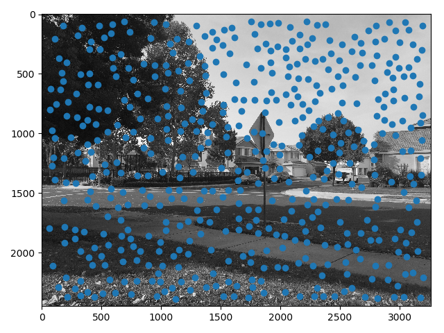
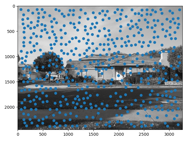
Part 2: Adaptive Non-Maximal Suppression (ANMS)

I implemented ANMS by sorting the points by their corner strengths. Then I calculated the radius of effect for each point using the sorted list, and then sorted the points again by radius. The first 500 points that had the highest radius of effect were selected to pass on to the next function.

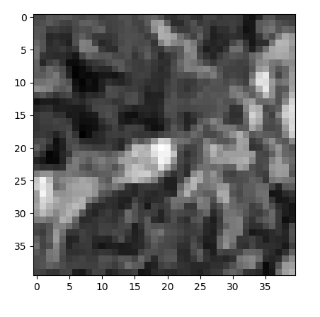
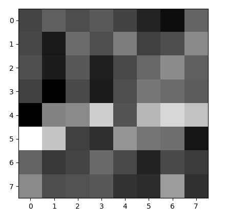
Part 3: Feature Descriptors

To create the feature descriptor patch for point, I sampled an area of size 40x40 around the point, then blur to a higher level of the gaussian pyramid, and downsample to an 8x8 patch. I then normalized the path, and flattened it to make calculating feature matches easier in the next step.

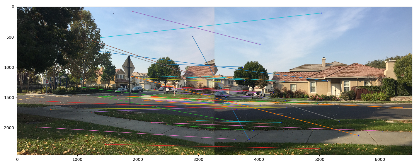
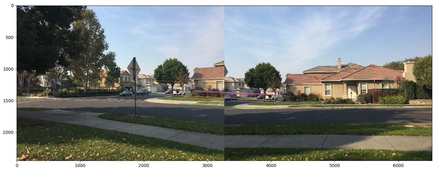
Part 4: Feature Matching

To match features, I computed the distances between every feature in image 1 and image 2. Then we found the minimum and second minimum distances and used the ratio between them to filter out matches. Because of the variance in these numbers, I decided to make the threshold set to the value of the 40th highest ratio, so that I would always get 40 matches.

As you can see, there are some correspondences in the results that should not be there. These will be removed in the next step.

Credits for the visualization code go to Ajay Ramesh at this Piazza Post.
https://piazza.com/class/jkiu4xl78hd5ic?cid=348

Part 5: RAndom SAmple Consensus (RANSAC)

RANSAC was implemented by picking four random sets of matched points, computing a homography for them, and seeing how many of the other points also fit this homography with an error less than a certain value. I chose 0.4 for this error threshold, and ran the algorithm for 8,000 iterations.

Credits for the visualization code go to Ajay Ramesh at this Piazza Post.
https://piazza.com/class/jkiu4xl78hd5ic?cid=348

Part 6: Results of Automatic Feature Matching

Below are the results of automatic feature matching.

One interesting thing to note is that the automatically matched features are generally just about as accurate as the manually matched ones. This is because the benefits of having a computer calculate the point correspondences and remove minute errors are balanced by the fact that I was really meticulous in choosing my points manually.

You can also see that the Playground image performed a lot worse with automatic matching. This is because the points of the trees that were moving in the wind also registered as features, and the homographies of the trees and the playground itself are slightly different. The algorithm was not able to warp to fit both, and so is stuck somewhere in the middle.

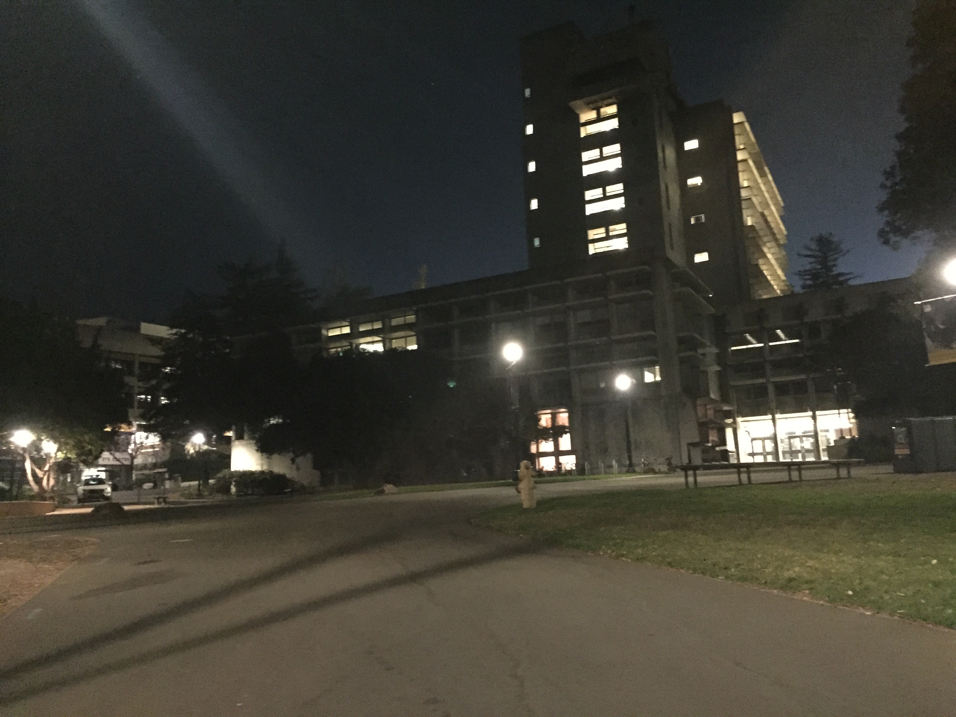
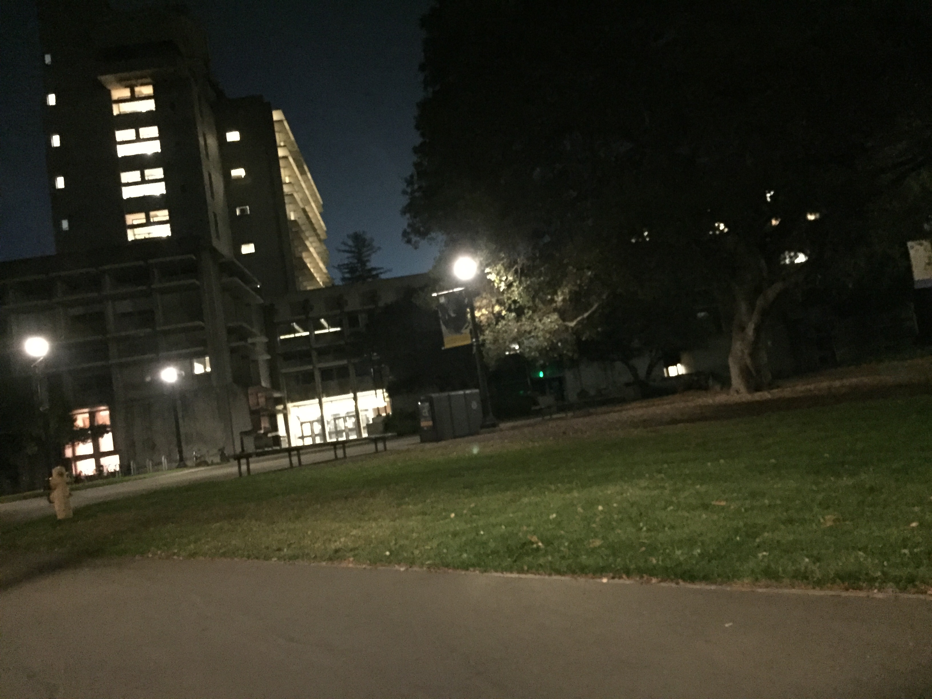
Another interesting thing to note is that the Night in Berkeley image was actually quite hard to get working, because of the presence of many similar-looking features in different places. I basically had to manually remove points and fine tune a bunch of parameters to get it to match up, so I suppose that one is less automatic than you'd think.

Part 7: What I have Learned

I really enjoyed this project! I thought it was awesome learning how automatic feature matching can be done, and I'm glad we started off with the easier bit first: I think it would have been a lot to do the whole automatic thing from the beginning. It also gave us a sense of how important it is to have accurate data.

I think the most interesting thing I learned was RANSAC. The method of computing the homography using four randomly chosen points, seeing how many other points fit, and then repeating this, is actually pretty simple, but really useful. This method "trying stuff and taking the best fit one," seems to have applications for other things as well.

Part 8: Multi-Scale Feature Descriptors and Corner Detection

I implemented multi-scale corner detection by forming a small gaussian pyramid over the image and calculating the harris corners at each level of the pyramid, then finding the unique corners in the combined list.

I implemented multi-scale feature descriptors by forming a small gaussian pyramid over each feature patch, normalizing each one, and then flattening and concatenating them to form feature vectors. I wasn't able to finish this part though, as the features didn't work very well. I tried many different sizes, but it only took much longer and produced no benefit.