[Auto]Stitching Photo Mosaics
CS194-26 Fall 2018
Bernie Wang
Part 1: Image Warping and Mosaicing
Overview
In this part, we explore the concepts of projective warping and applying those by composing panoramas. The goal is to compute homographies for two or more images, warping them onto the same projective plane, and blending the images together. We can also use the same technique for computing homogaphies to rectify the projective plane of an image.
Shoot the Pictures
All the pictures displayed in this project were shot using an iPhone 6S by yours truly. For images used for composing the same mosaics I tried my best to rotate the camera about a vertical axis without translating the camera. This will result in better panoramas because the computed homographies will better model the projection from one plane to another.
Recover Homographies
In order to project an image onto a projective plane, we use the following homography matrix:
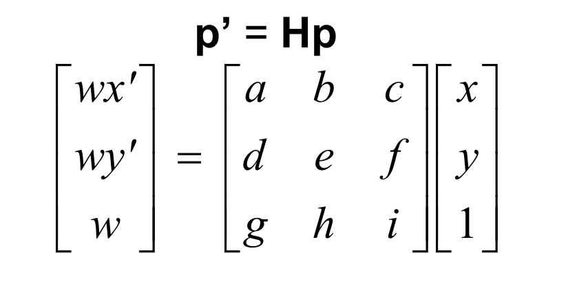
Homography matrix
To compute the homography matrix, we sample some correspondence points between two images and then use linear least squares regression to solve for the matrix that fits best.
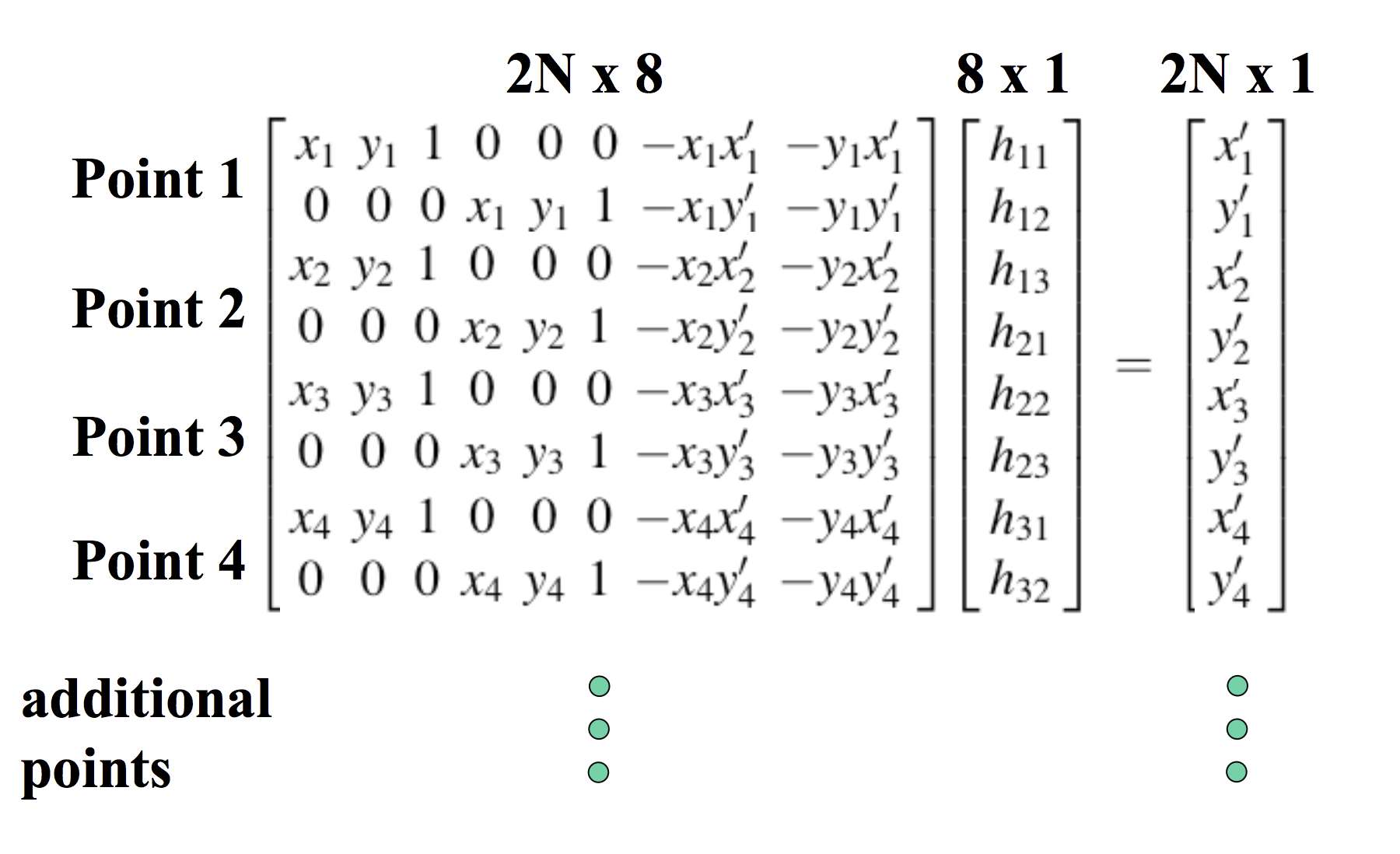
Image from Robert Collins
Warp Images
After we have computed our homography matrix, we can warp our image. We will use the reverse warping approach. We first compute the forward warping from the source image to the target image to get the bounds of the projected image. Then, we get all the points bounded in our projected image and use the reverse homography and interpolation to get the respective pixel values.
Image Rectification
We can demonstrate image warping by "rectifying" the projective plane to be frontal-parallel. We can do this by corresponding some boundary points in our source image to boundary points on a rectangle, compute the homography matrix, and warp our source image.
Original
Rectified, cropped
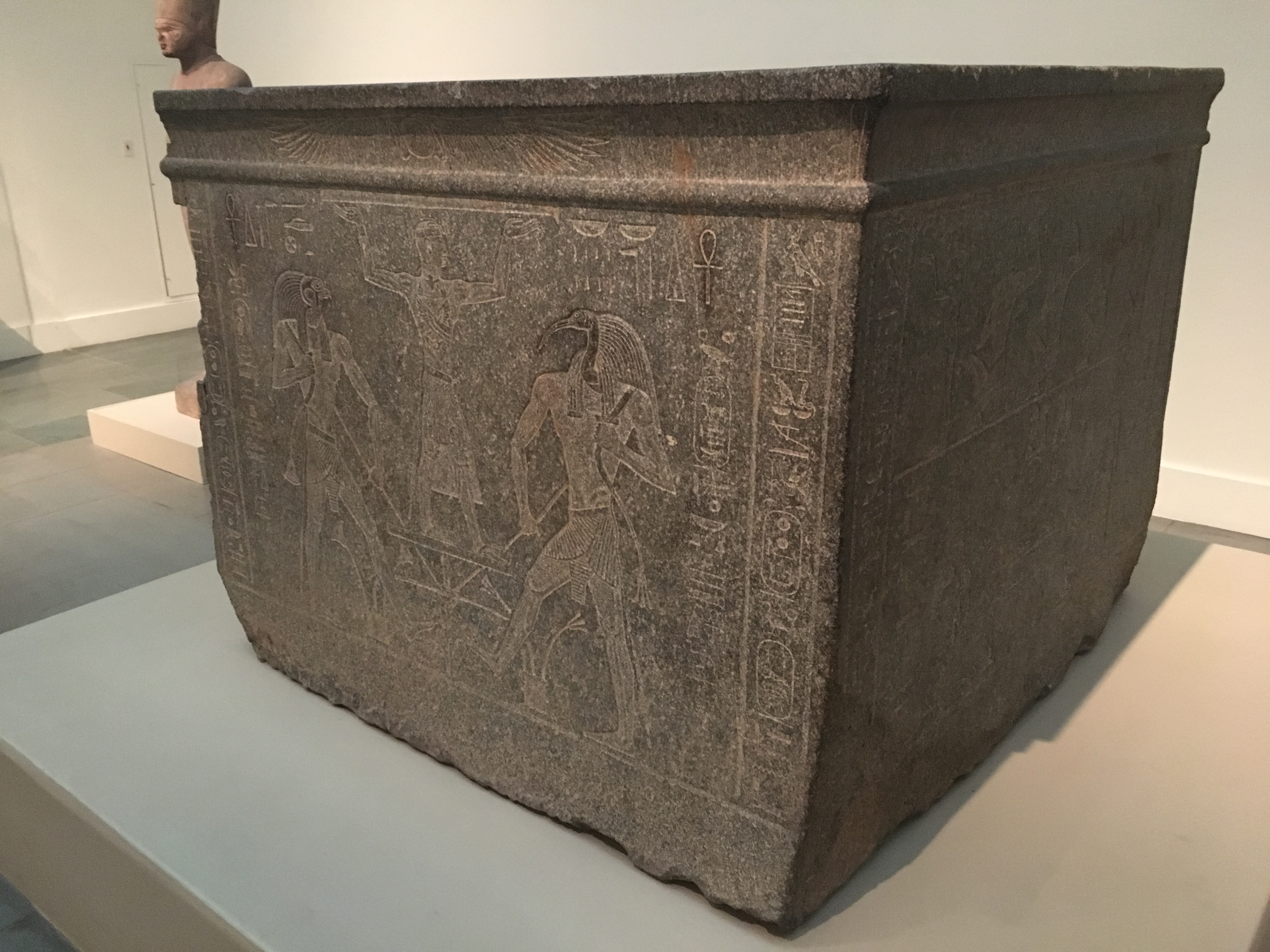
Original
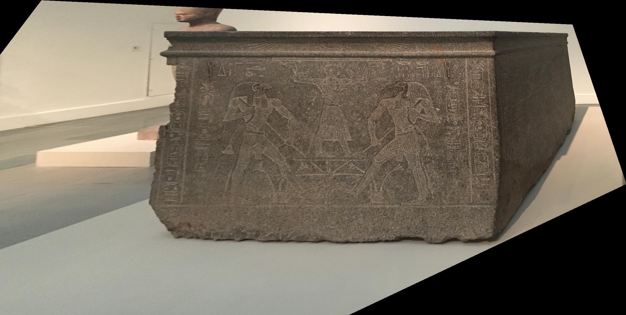
Rectified, cropped
Blend the images into a mosaic
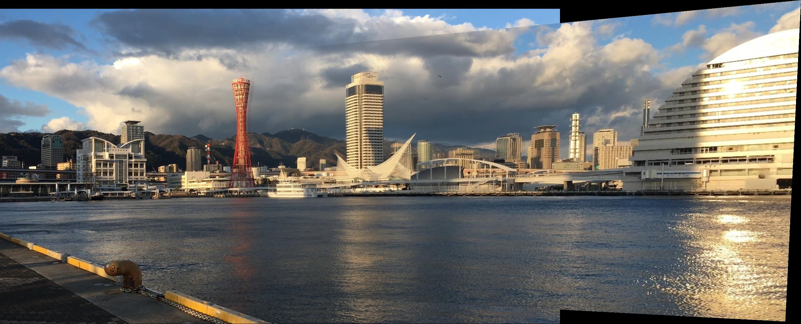
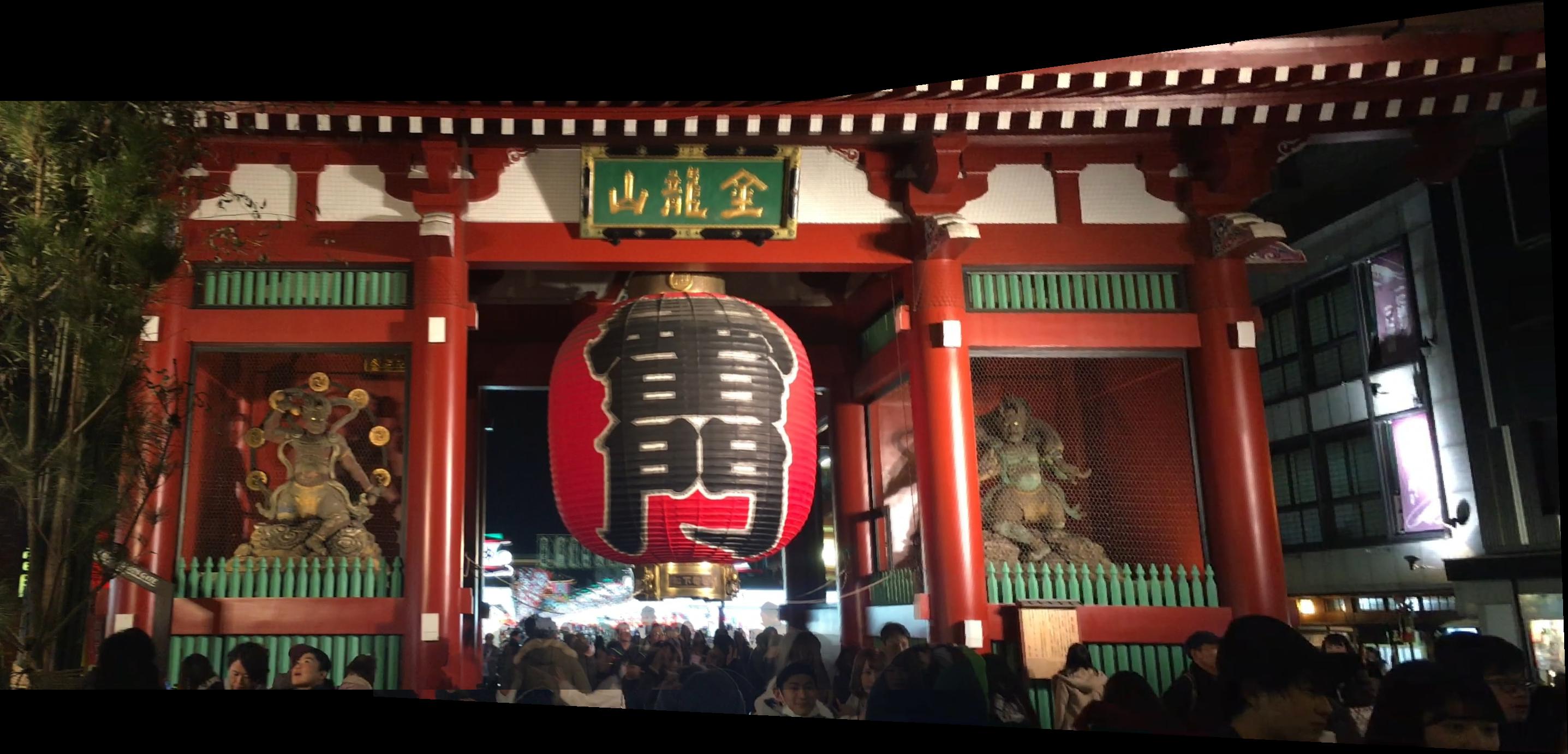
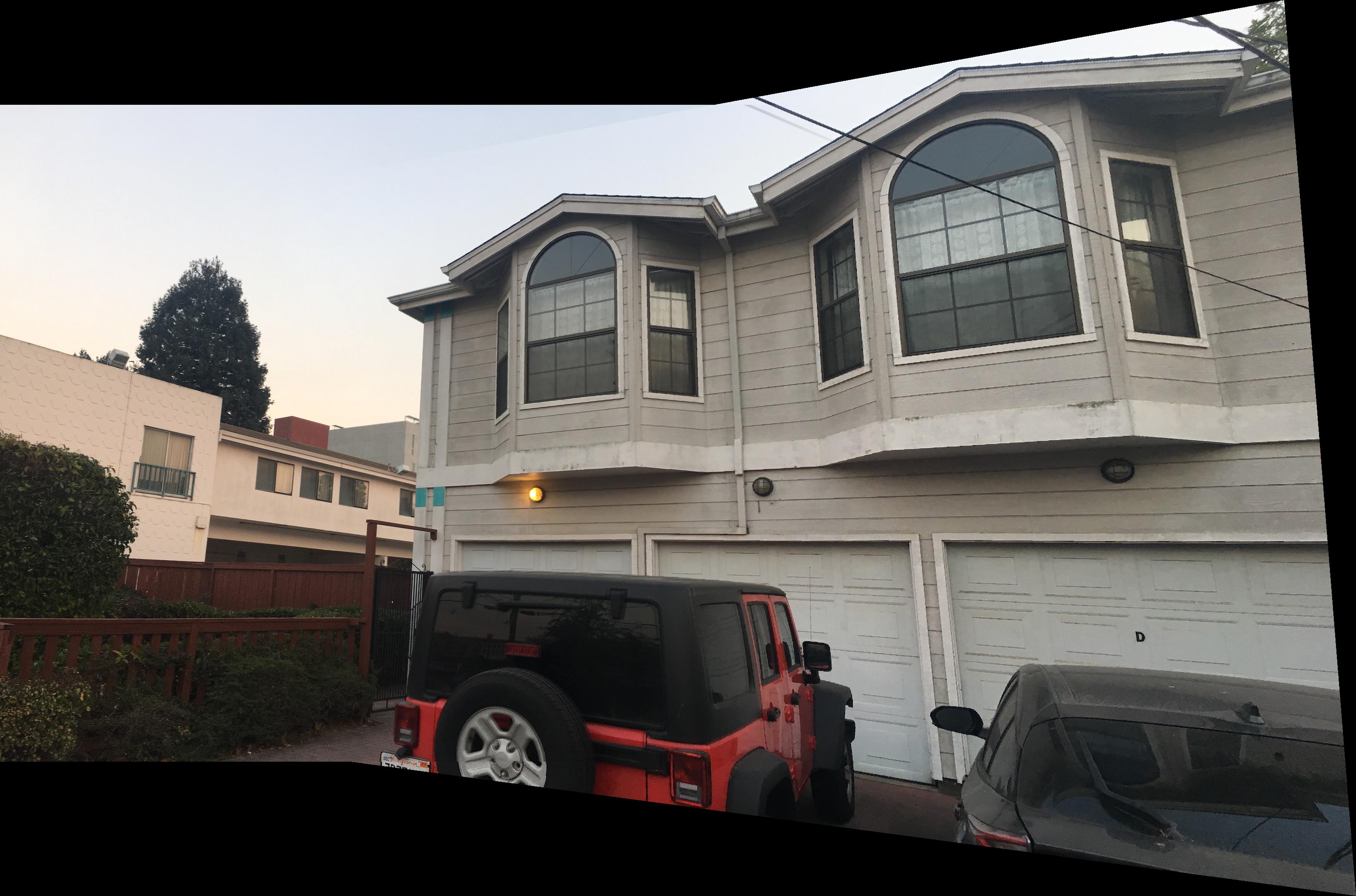
Now we can use warping to create mosaics! First we get correspondence points between two images, and warp one of the images onto the projective plane of the other. Then, we realign the images so that the correspondence points overlap. Lastly, we use linear blending to stitch together the images. The challenge in using linear blending is to only scale pixels in the overlapping region, so we needed to find the pixels that lie in the overlap.
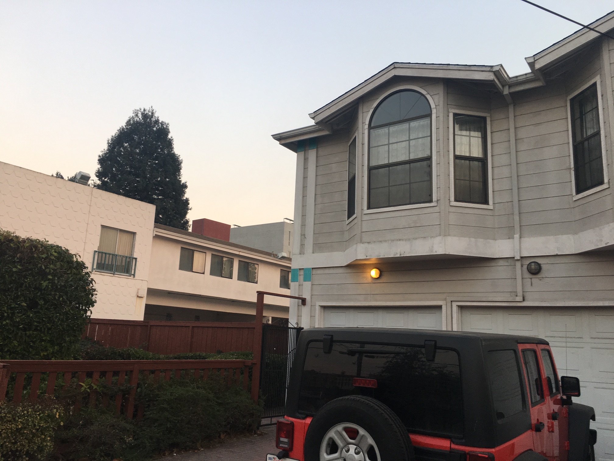
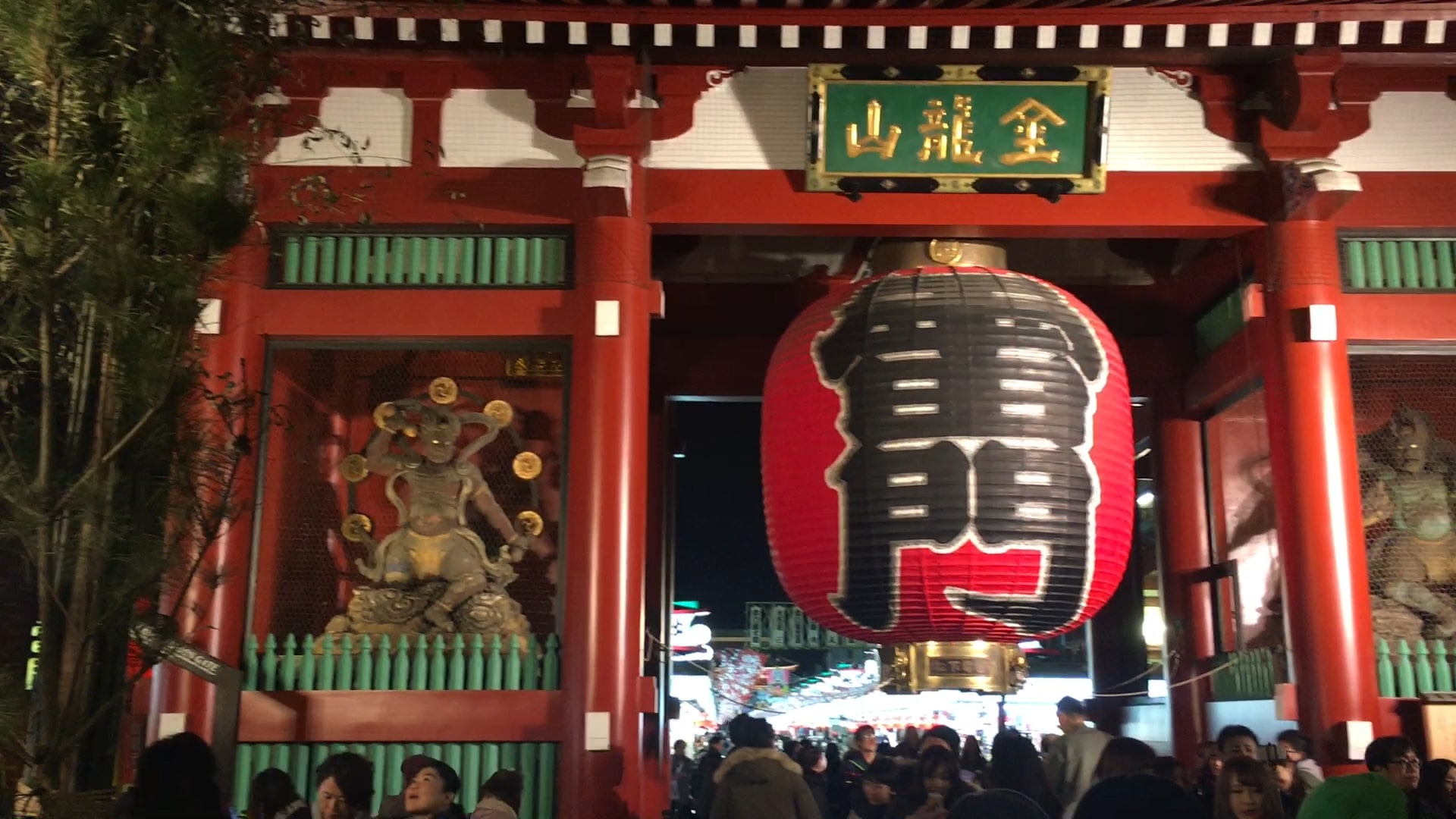
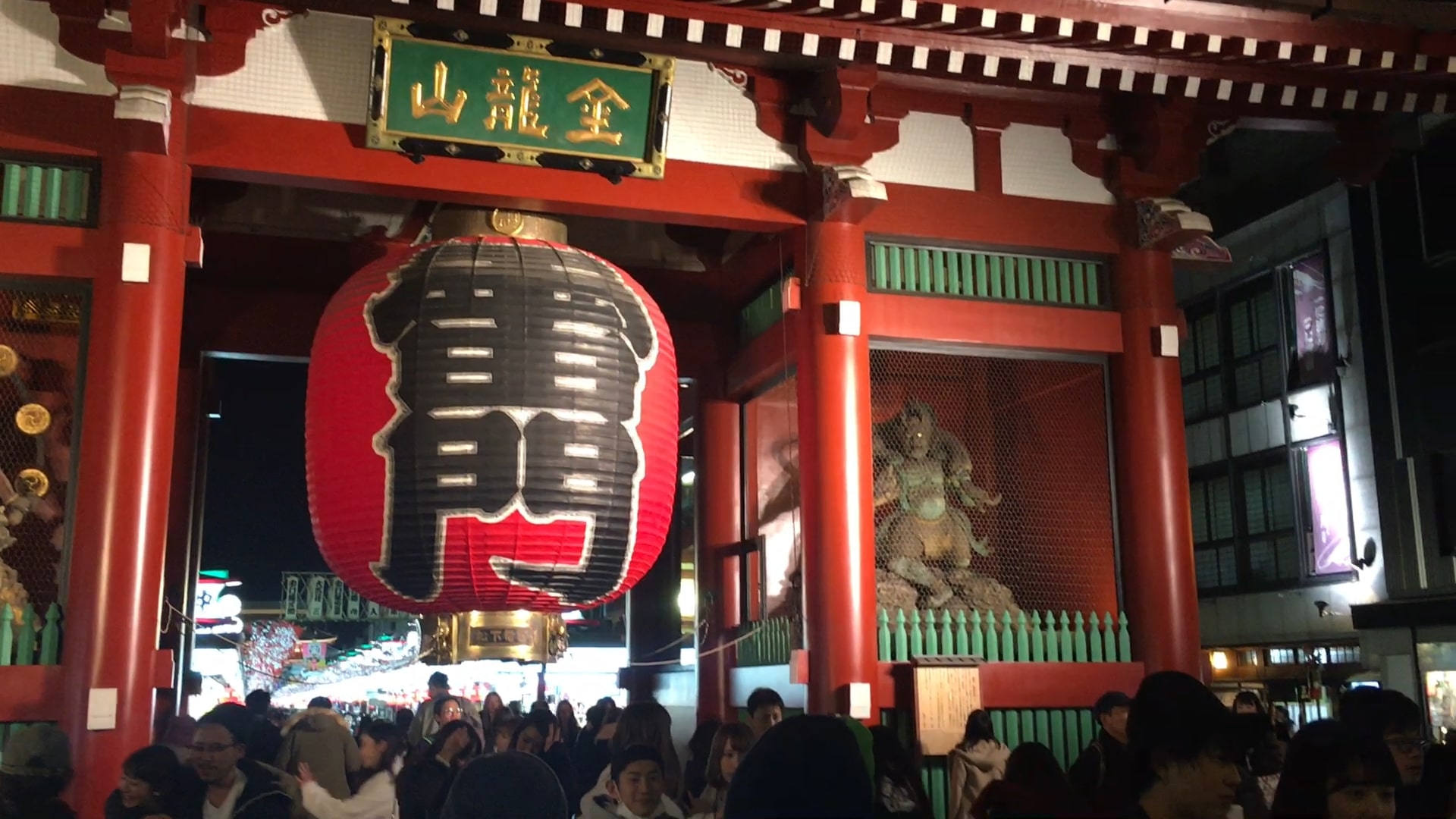
Original
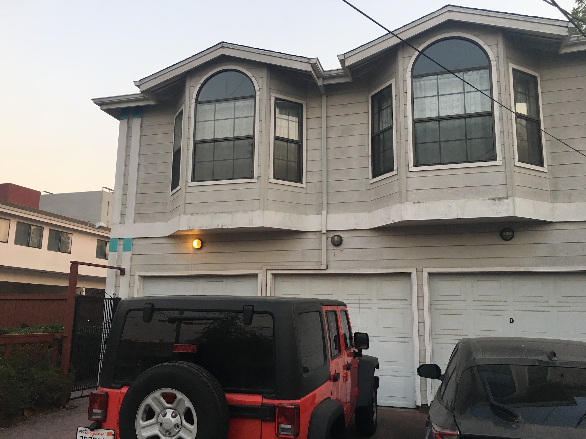
Original
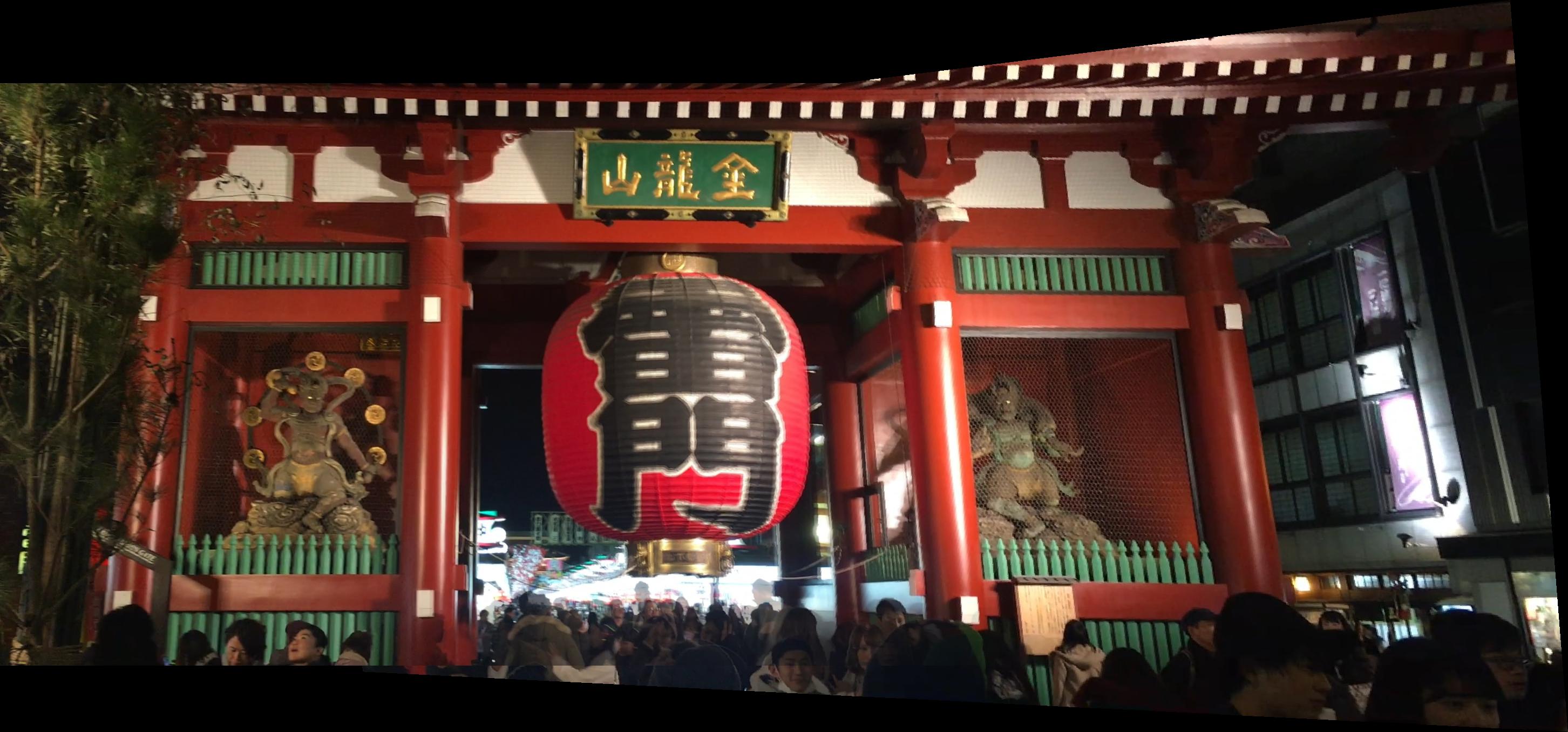
Mosaic

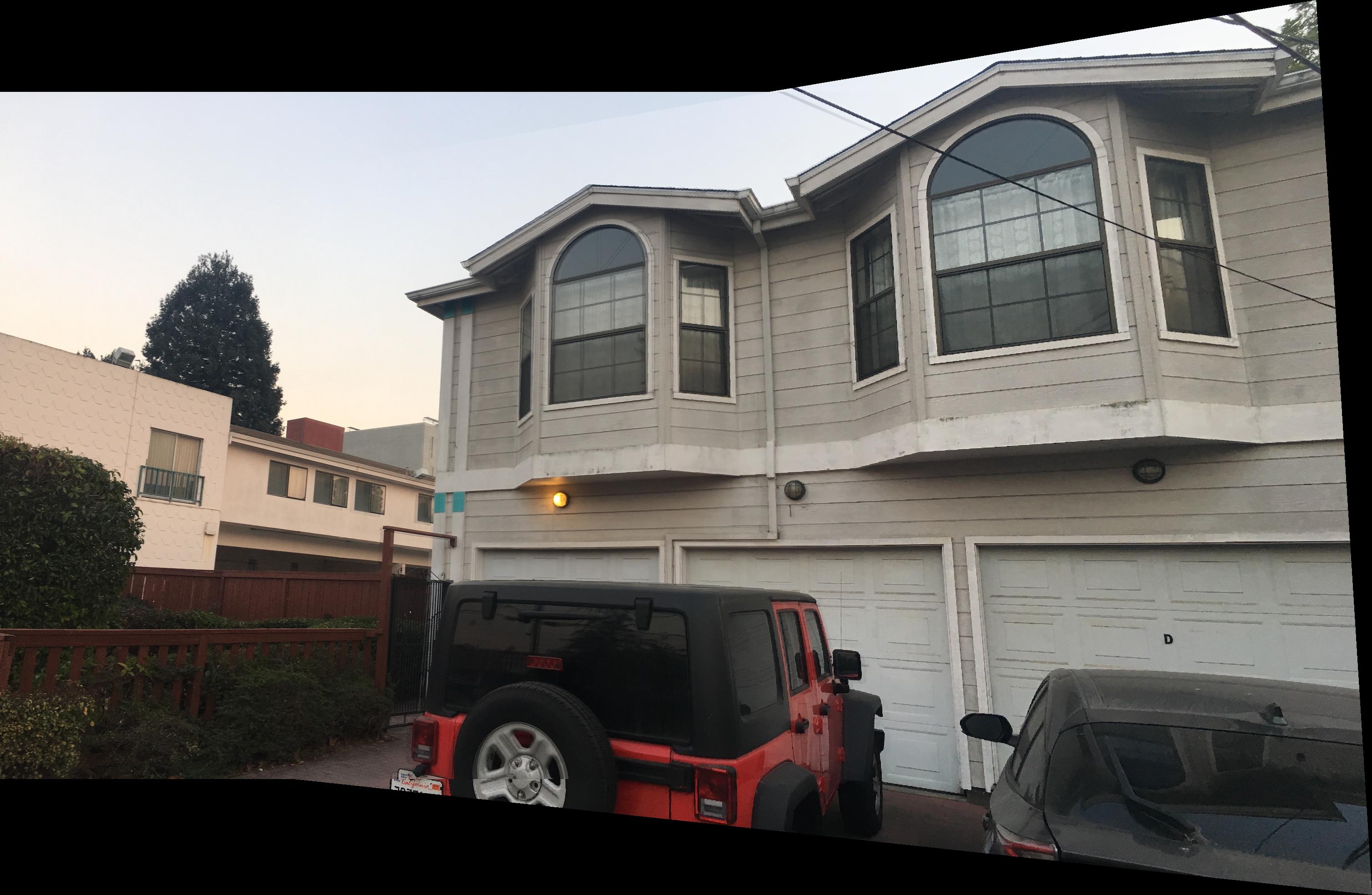
Original
Original
Mosaic
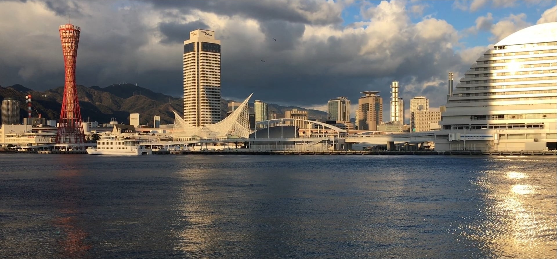
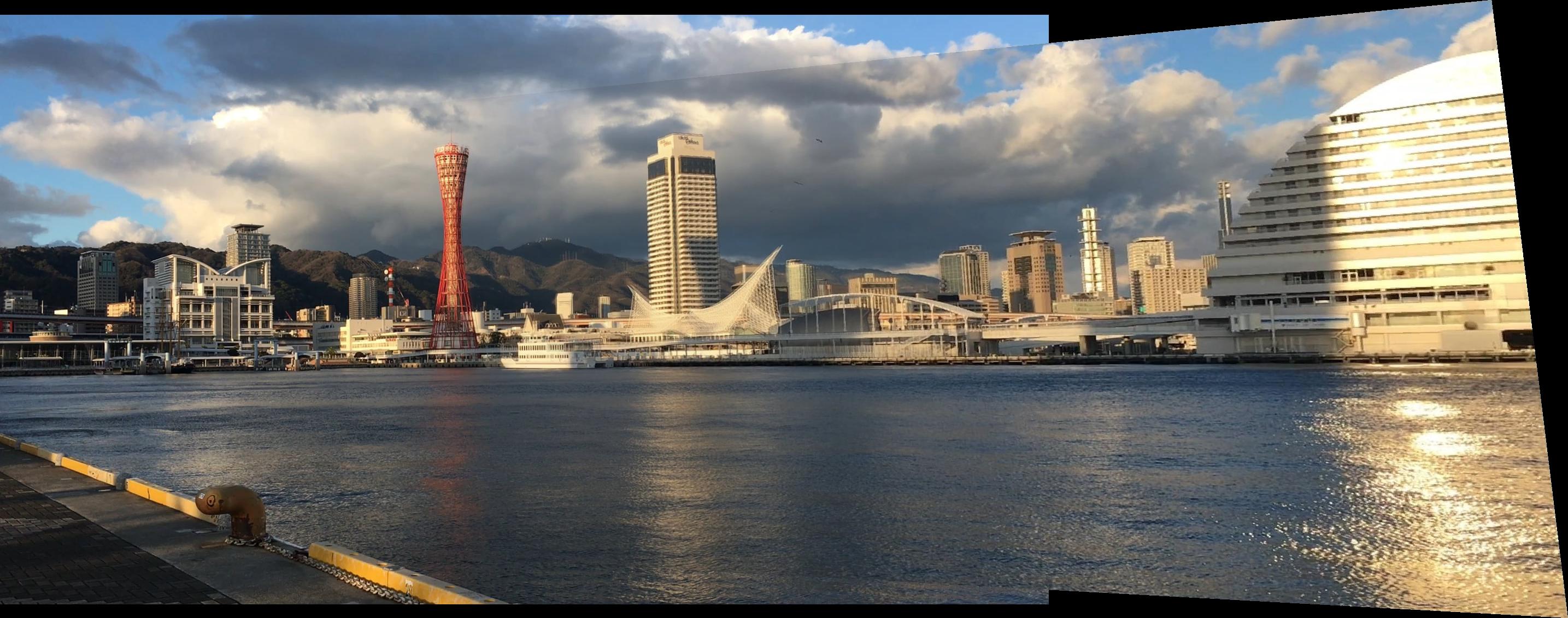
Original
Original
Mosaic
What I learned
I learned how getting the small details correct makes a big difference in the visual quality of panoramas. For example, having accurate correspondence points makes all the differences in aligning images. Once you can find out how to align and blend images correctly, you can make some beautiful panoramas!
Part 2: Automatic Stitching
Overview
Hand labelling correspondence points is tedius and often times inaccurate. In this part we will implement the paper “Multi-Image Matching using Multi-Scale Oriented Patches” by Brown et al. with several simplifications.
Detecting Corner Features in an Image
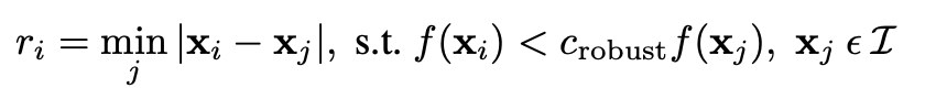
Corner points are good candidates for correspondence points. In this part we use Harris corner detection to corners, or points whose neighbors lie in different edge directions. In order to reduce the number of corner points detected I set the minimum distance threshold for finding the peak local maximum to be 15. Below is an example of corner points detected overlayed on the source images.
Extracting a Feature Descriptor for Each Feature Point
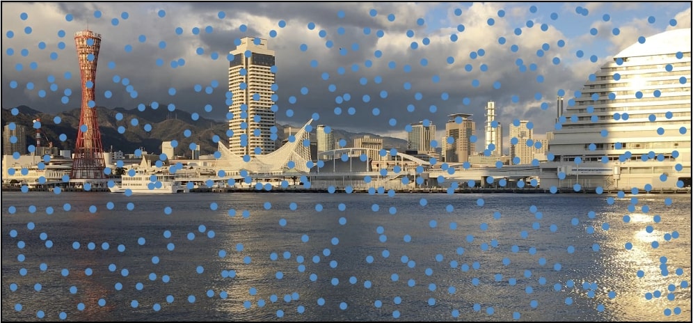
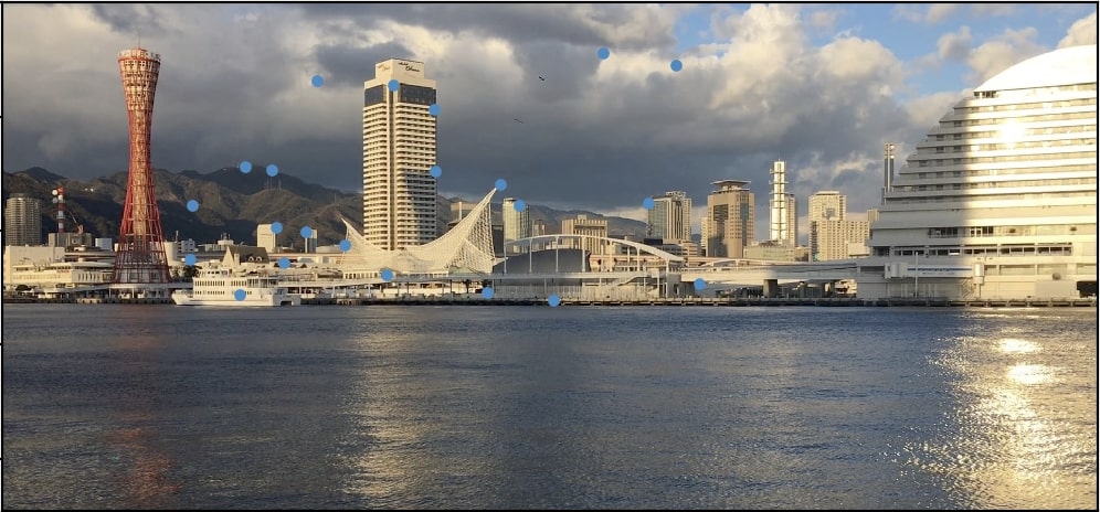
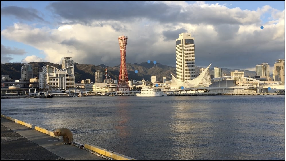
Although the Harris corner detection algorithm will find corner points, it is desirable to keep only a certain number of points for computational efficiency down the line. However, we also want the remaining points to be spatially well distributed. To solve this problem we implement adaptive non-maximal suppression (ANMS) which selects the points with the top-k largest minimum suppression radius. The minimum suppression radius can be found by solving the following equation:
Minimum suppression radius
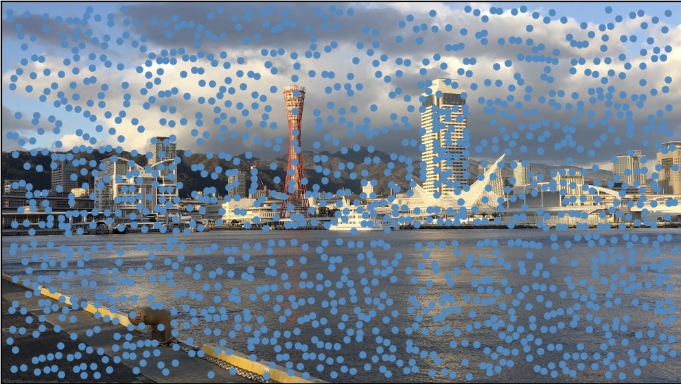
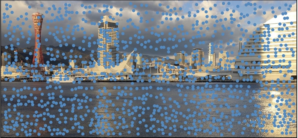
Here, we choose 500 corner points to keep and overlay them onto the source images:

Matching These Feature Descriptors Between Two Images
Now that we have our interest points, we can use them as feature descriptors for our source images. We create a 41 x 41 patch centered about each of our interest points, smooth them with a gaussian filter, and downsample them to 8 x 8 patches. We then calculate their respective Lowe ratio by getting the SSD of their 1-NN and their 2-NN. By thresholding the interest points by their Lowe ratio, we get feature matches between our source images. Below is an example of some matches:

Use a Robust Method (RANSAC) to Compute a Homography
The feature matches from above look good, but you can tell there are some outliers. To correct this, we run RANSAC (random sample consensus) to get the largest set of inliers. It first randomly selects 4 pairs of matches and then compute a homography matrix out of them. Then is projects features from one image to another, and by calculating the SSD of the projected features and the actually features and thresholding, we can get a set of inliers. We do this for many iterations (in the below case 1000) and choose the largest set of inliers to compute the actual homography matrix use for mosaicing. Below are the inliers found by RANSAC:

Results
Below are some examples of mosaicing. The left side is from manually labelling correspondence points and the right is from automatic feature matching:
Manual labelling
Automatic labelling
Manual labelling
Automatic labelling
Manual labelling
Automatic labelling
What I Learned
I was suprise by how robust automatic feature matching was. I have already learned some of the algorithms used in the project like RANSAC from research but I learned how Adaptive Non-Maximal Suppression can be useful for sampling points and also how important choosing the right thresholds is for getting good results.