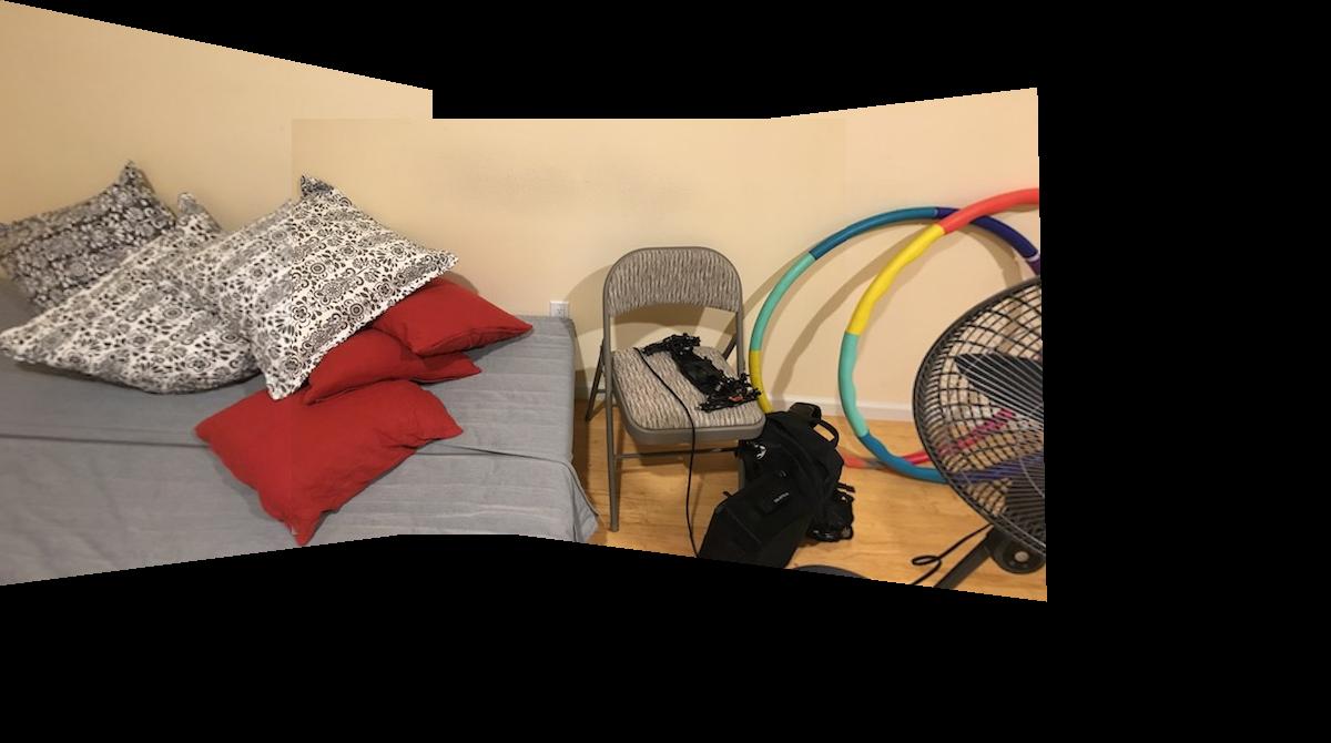
Part 2: Recover Homographies
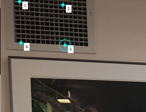
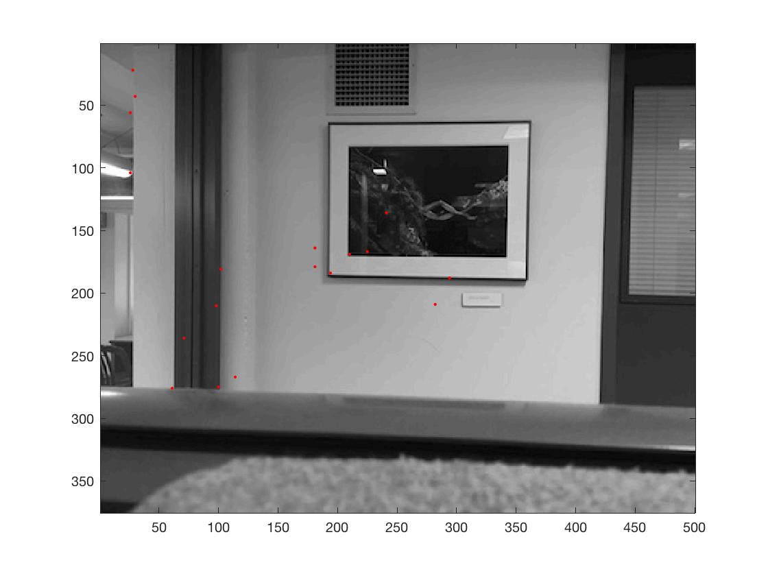
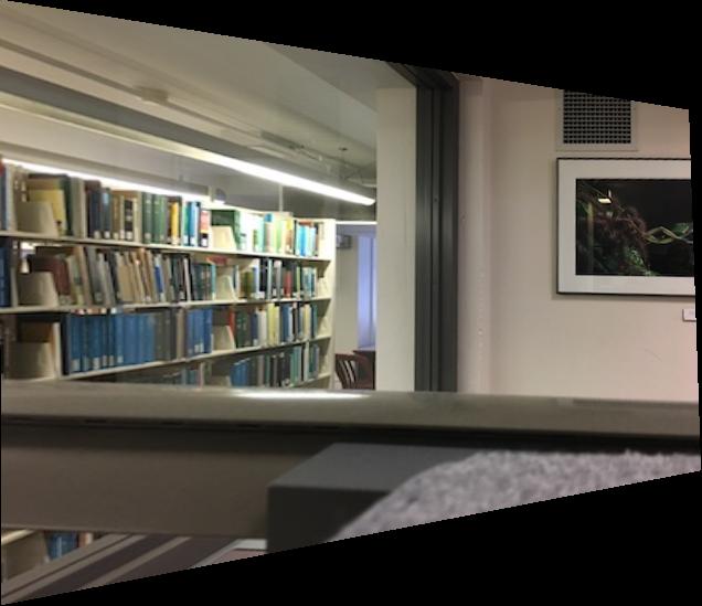
In this part, I used the method outlined in this post, which is basically computing the w for each individual point, and scaling the previous two equations. Therefore, there are two equations for each pair of points. For this part, I picked 9 coorepondences between q1.jpg and q2.jpg, and 10 coorespondences between q2.jpg and q3.jpg. Then I use least square solver to find the optimal a-h parameter, to reconstruct the H matrix.
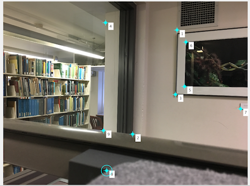
q1 points - 1_2
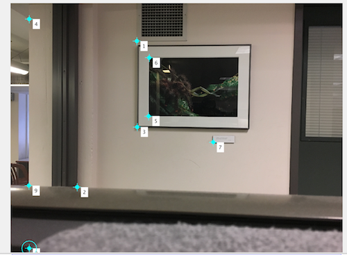
q2 points - 1_2

q1 points - 3_2
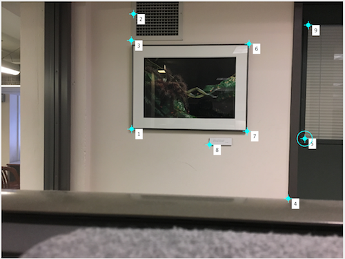
q2 points - 3_2
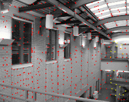
Part 6: Detecting corner features in an image
For this part I first ran the included Harris Corner Detector on the image
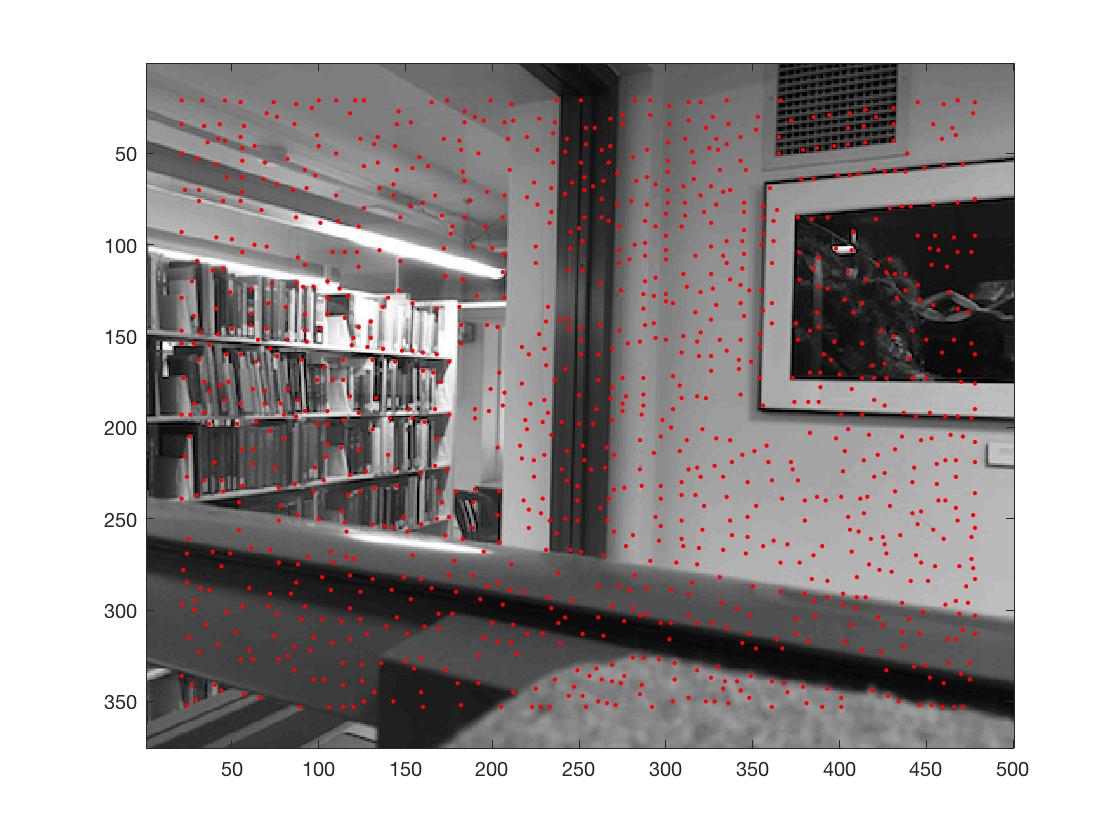
q1.jpg with Harris Corner Detector
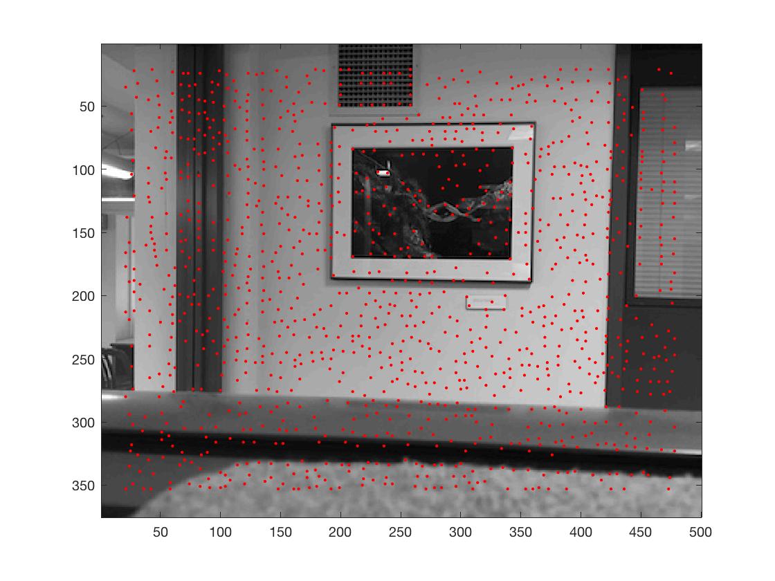
q2.jpg with Harris Corner Detector
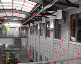
Then I follow the ANMS formula as descriped in the paper. To improve efficiency, I decided to manipulate the order of the formula, and calculate a threshold for each point x_i, and compute the minimum for all the points that meet the threshold. In the end, I sort the points by radius and took the top 500 for matching
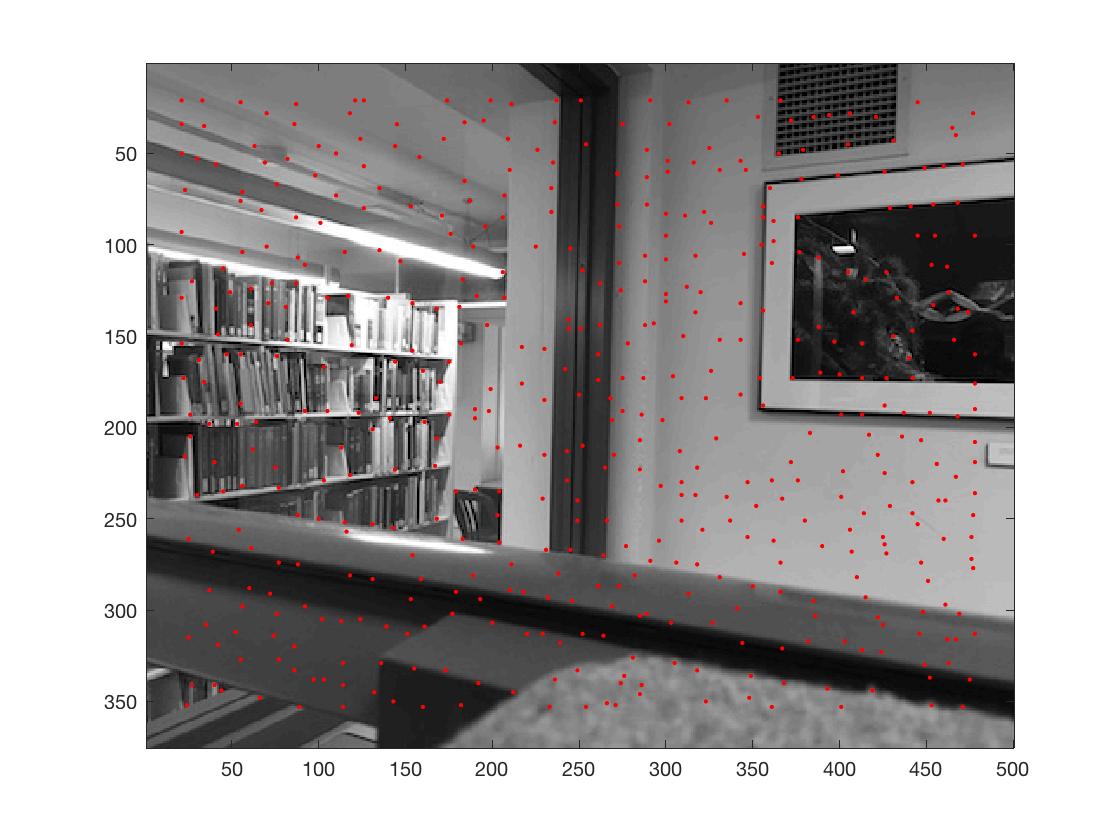
q1.jpg with Harris Corner Detector
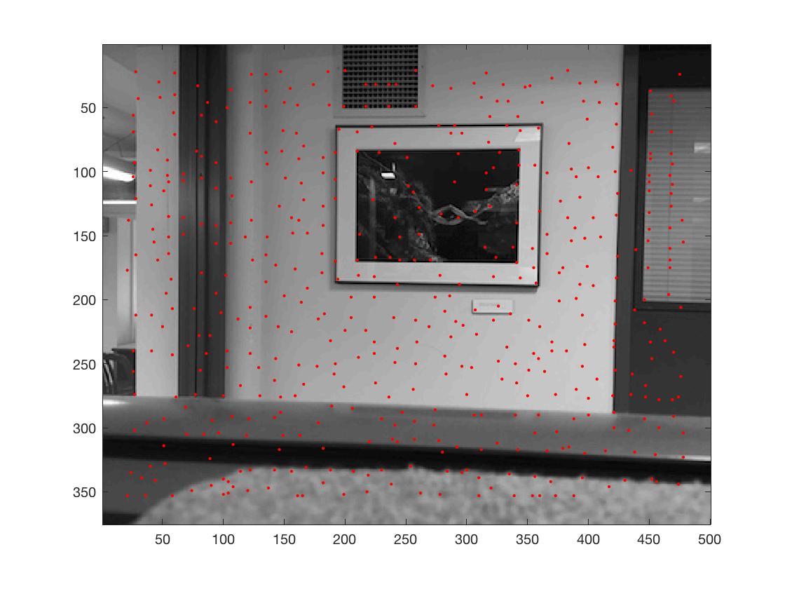
q2.jpg with Harris Corner Detector
Part 6: Tell us what you've learned
Matlab is tricky. X and Y coordinate can cause many troubles if one is not careful. In addition, selecting points that spread across the image will result in better homography. Last but not least, keeping track of extra information about offset when shifting is the way to go.
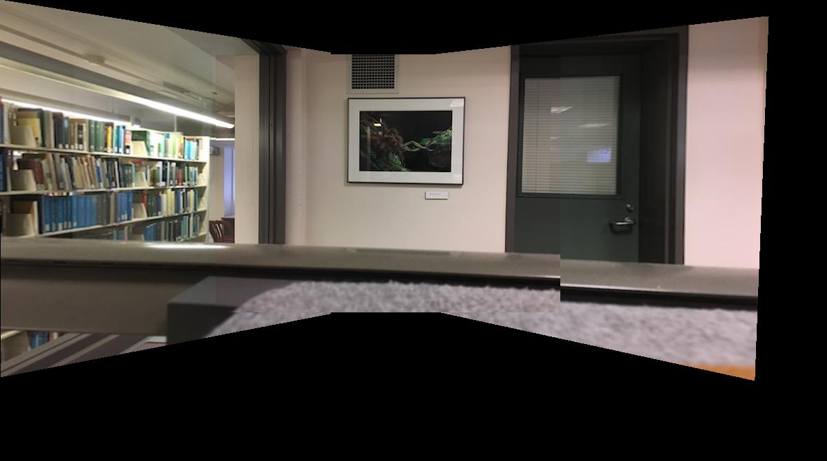
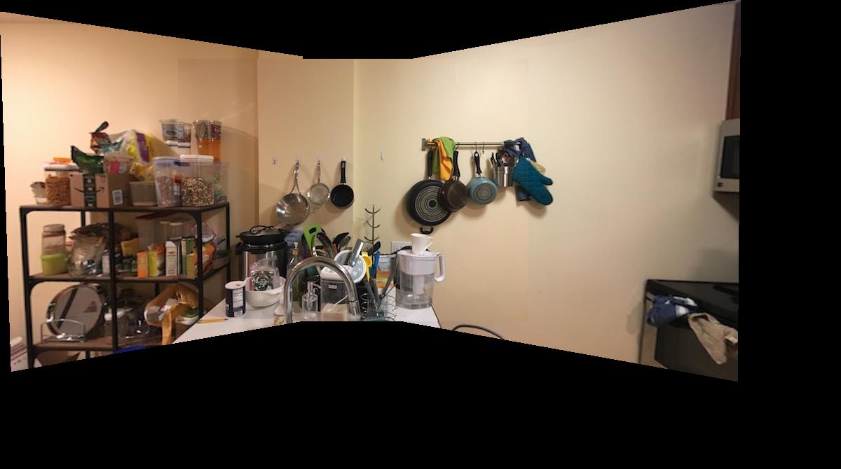
However, auto-mosaicing is so much cooler! No more hand selection needed! Wahoo!!!