CS 194-26 Project 6: Image Warping and Mosaicing (Part 1)

This is the submission of Myron Liu (cs194-26-afp) for CS 194-26 Project 6: Part 1.

Part 1 Shoot and Digitize Pictures Homography Recovery Image Rectification (Warping Images) Image Blends (Image Stitching) Summary

Part 2 Detecting Harris Corner Features Extracting Descriptors and Matching RANSAC Automatic Image Stitching Summary

Part 1

Background

In this project, we digitize pictures and use homography to projectively warp images, resampling them and finally compositing them into an image mosaic.

Shoot and Digitize Pictures

These images were taken with a DSLR. The first set were taken at a trip I took to Santa Cruz, the next set at Hearst Mining Circle, and the last set was taken of some random cars.

Santa Cruz Apartment Home Part 1

Santa Cruz Apartment Home Part 2

Santa Cruz Apartment Home Part 3

Hearst Mining Circle Part 1

Hearst Mining Circle Part 2

Hearst Mining Circle Part 3

By Car Part 1

By Car Part 2

By Car Part 3

Homography Recovery

By defining point correspondences between two images, we can define a transformation from one image to the other. Specifically, we find 8 unknowns using at least 4 points correspondences to recover a 3x3 homography matrix - this can be done using least-squares with an overdetermined system with more than 4 point correspondences.

Image Rectification

We can use the homography calculated from defining points correspondences to produce shifts in perspective in images. Below are some images produced from shifting perspective by computing a particular homography on an image and applying the homography.

Picasso Girl With Mirror (Side Perspective)

Chosen Points on Original Image (Rectifying to Flat Quadrilateral Plane)

Rectified Picasso Girl With Mirror

Hallway (Frontal Perspective - Angled Over Rug)

Chosen Points on Original Image (Rectifying to Flat Quadrilateral Plane)

Rectified Rug With Birds-Eye-View Perspective

Image Blends

After performing the transformation on the image, we stitch together images using translation without blending, alpha blending and Gaussian blending below.

Hearst Mining Circle Part 1 Point Correspondences

Hearst Mining Circle Part 2 Point Correspondences

Hearst Mining Circle Part 1 Homography Applied

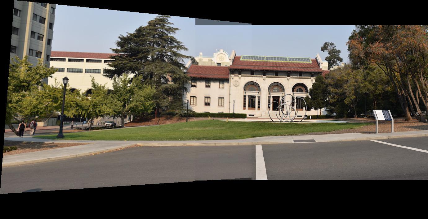
Hearst Mining Circle Part 1 + Part 2 Without Blending

Hearst Mining Circle Part 1 + Part 2 Linear Alpha Blending

By Car Part 1 + Part 2 Without Blending

By Car Part 1 + Part 2 With Linear Alpha Blending

Santa Cruz Apartment Home Part 1 + Part 2 Without Blending

Santa Cruz Apartment Home Part 1 + Part 2 With Linear Alpha Blending

Summary

I learnt about using homographies to transform the perspective of images and that blending properly for images is very hard - especially when you are choosing point correspondences manually.

Part 2

Harris Corner Detection

Using Harris Corner Detection kindly supplied by Professor Alexei Efros. Below are images that have had points of interest detected via Harris Corner Detection. Then the number of points is curbed down to 500 using Adaptive Non-Maximal Suppression (ANMS). The methods used are described in sections 2 and 3 of this paper.

Hearst Mining Circle Part 1 Harris Corner (without ANMS)

Hearst Mining Circle Part 1 Harris Corner (with ANMS)

Hearst Mining Circle Part 2 Harris Corner (without ANMS)

Hearst Mining Circle Part 2 Harris Corner (with ANMS)

Extracting Descriptors and Matching

At each interest point remaining from the above steps, we compute a 40x40 pixel window for each point, apply a Gaussian blur and resize to an 8x8 pixel block. Then correspondences are defined between the two images and only points a 1-NN/2-NN below a defined threshold are accepted. The methods used are described in sections 4 and 5 of this paper . Below are results between the Hearst Mining Circle Part 1 and Part 2 images at different threshold c values - the visualization code was provided by Ajay Ramesh.

Hearst Mining Circle Correspondences: c = 0.8

Hearst Mining Circle Correspondences: c = 0.6

Hearst Mining Circle Correspondences: c = 0.4

RANSAC

As we can see above, when we set c = 0.4, we get a decent number of correspondences to perform a homography between the two images. However, we still have some correspondences that will lead the homography to produces large errors. Thus we apply the RANSAC technique to further cut down the number of correspondences - we compute a homography between 4 points chosen randomly from the set of points after the above results. Then we check the deviation of the actual points from the calculated point from the transformation and add the points to the final set of correspondence points depending on a chosen threshold value. Below is the final automated correspondence points.

Hearst Mining Circle Correspondences After RANSAC

Hearst Mining Circle Part 1 Correspondences

Hearst Mining Circle Part 2 Correspondences

Automatic Stitching

After obtaining the correspondences automatically, we can apply the algorithms used in part 1 to perform automatic stitching to build a panorama. Below are the results of following automatically calculated correspondences, their computed homography applied on the image and the final stitched image using linear blending.

Hearst Mining Circle Correspondences After RANSAC

Hearst Mining Circle Part 1 With Homography Applied

Hearst Mining Circle Part 1 + Part 2: Linear Alpha Blending (Compare with manually choosing correspondences above in part 1)

Car Correspondences After RANSAC

Car Part 1 With Homography Applied

Car Part 1 + Part 2: Linear Alpha Blending (Compare with manually choosing correspondences above in part 1)

Home Correspondences After RANSAC

Home Part 1 With Homography Applied

Home Part 1 + Part 2: Linear Alpha Blending (Compare with manually choosing correspondences above in part 1)

Summary

I learnt about Harris Corner detection along with feature matching can be a really neat way to automatically detect and recognize important points in images. Combining a lot of different data processing techniques and thresholding - you can lower a noisy set of data points into something very useful which can be applied with techniques like image stitching to produce wonderful effects.