CS194 Project 6A, Nikhil Patel
Summary
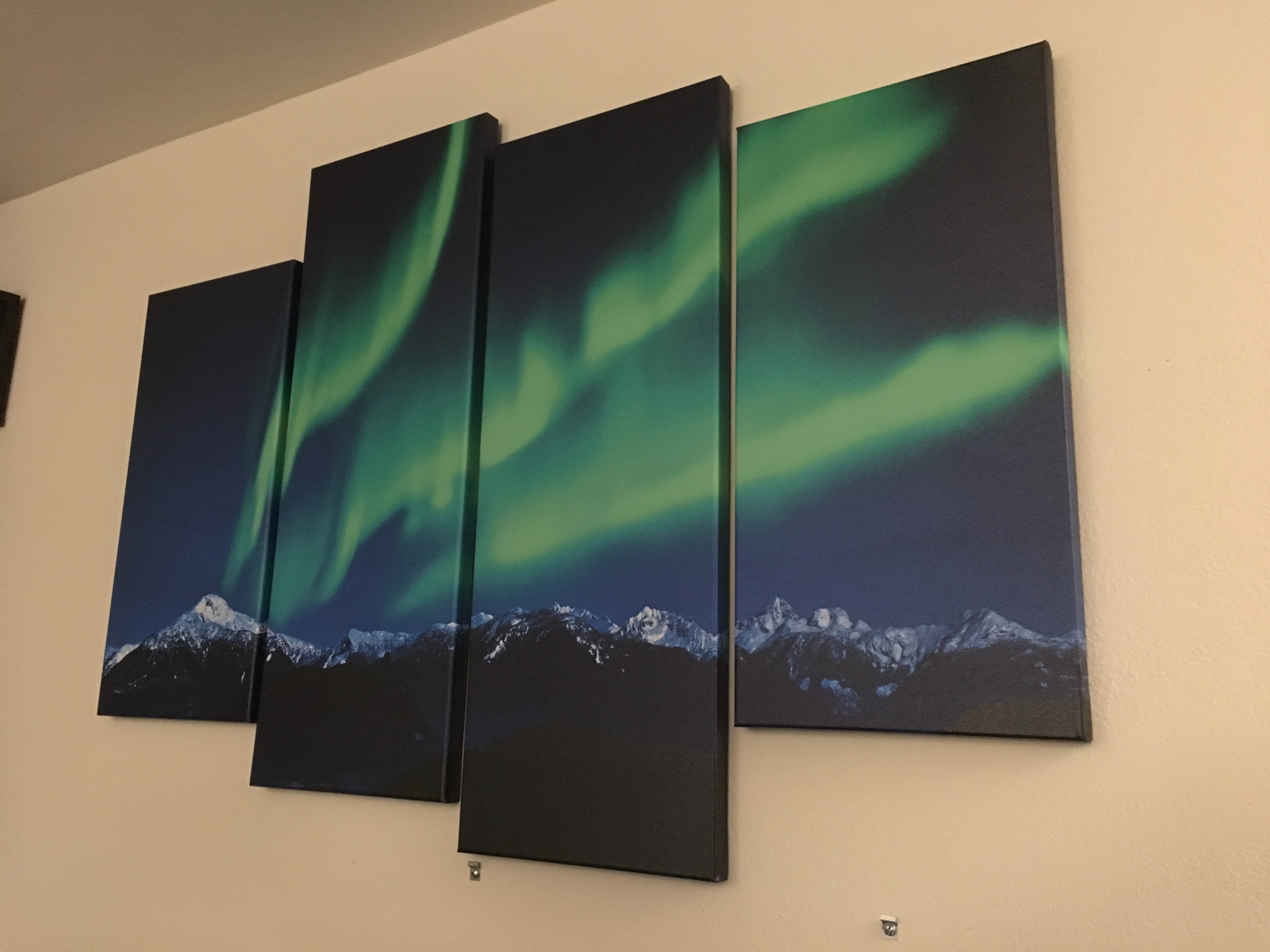
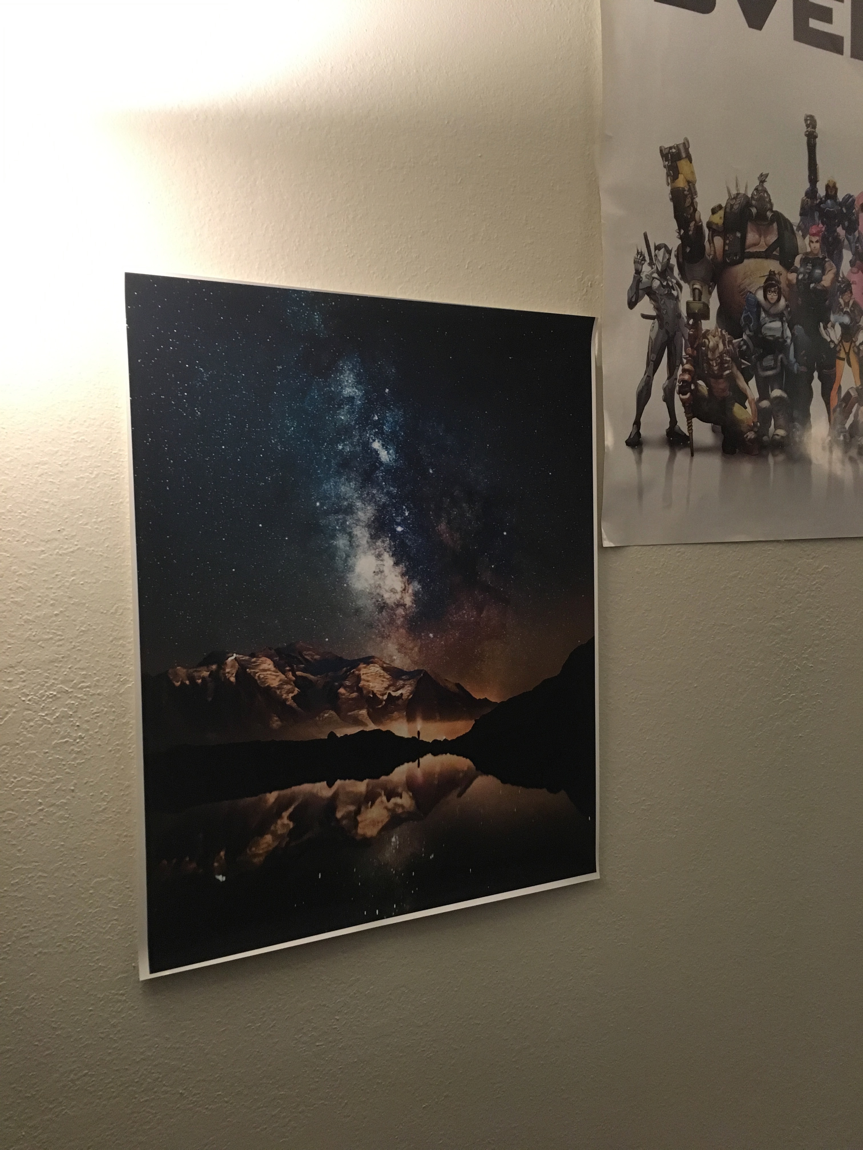
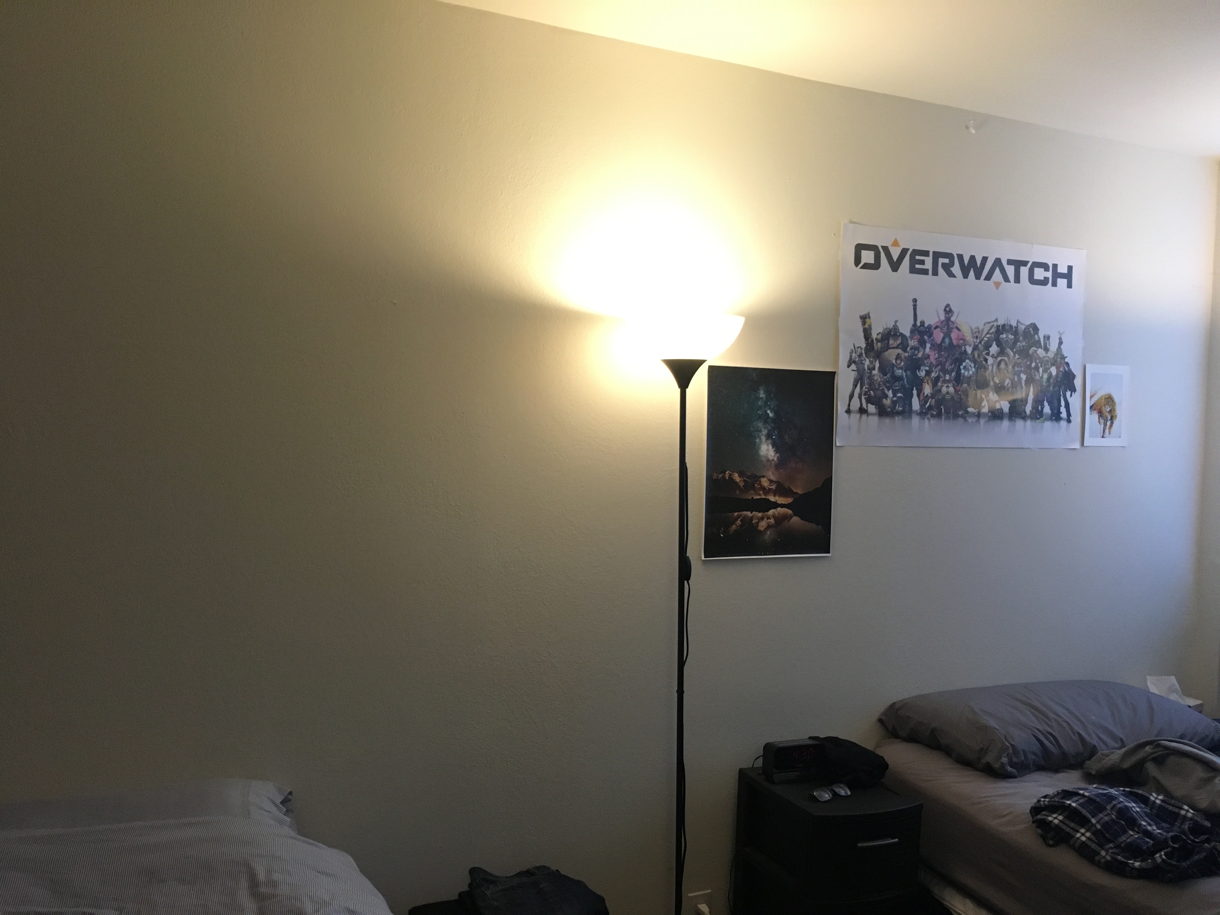
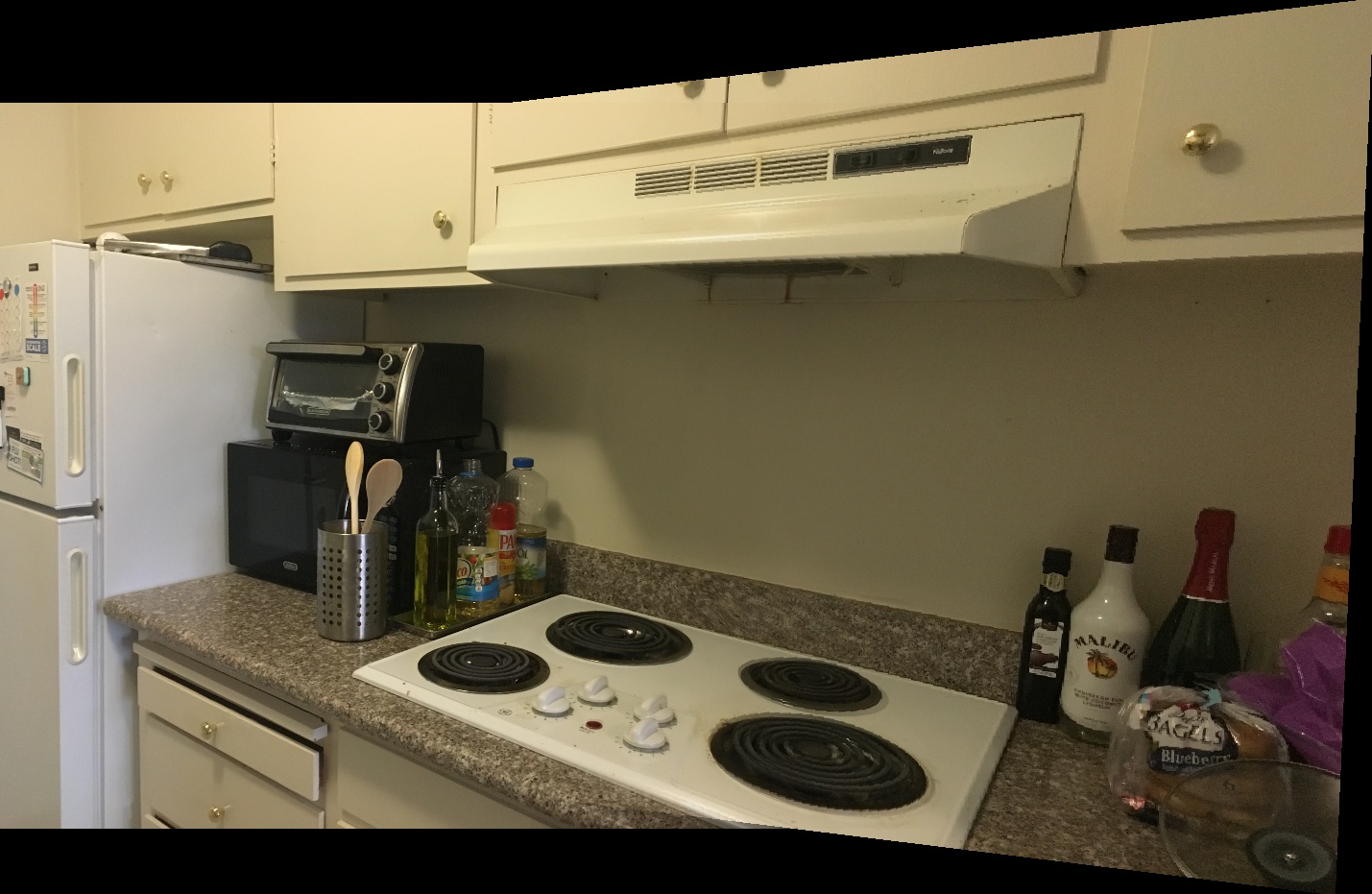
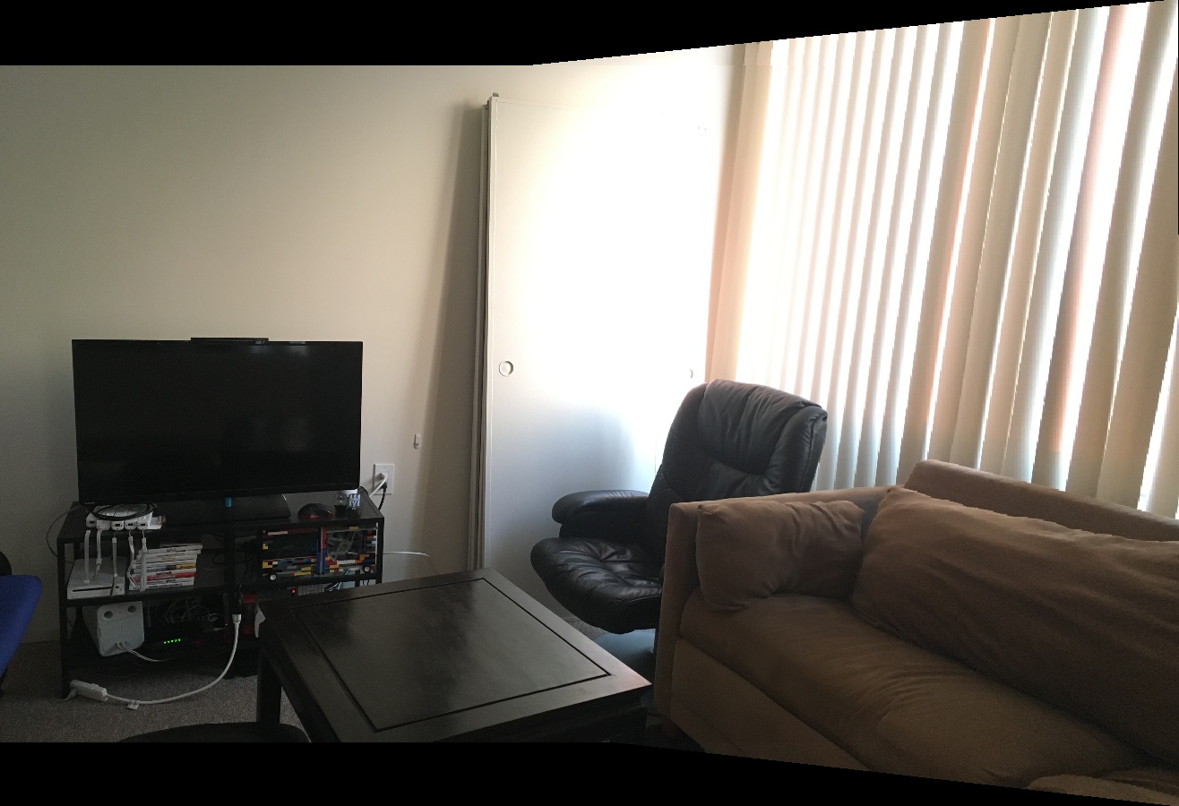
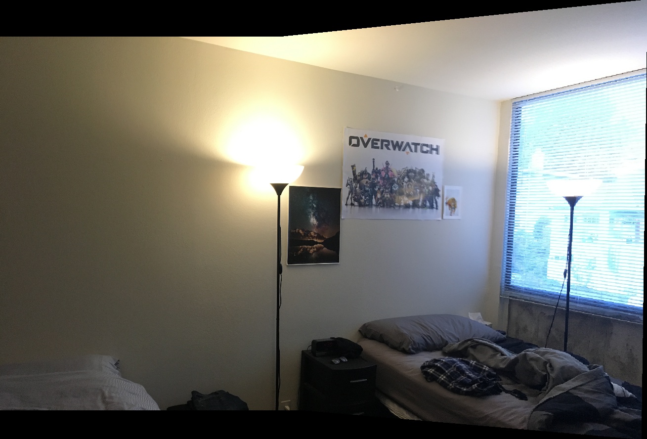
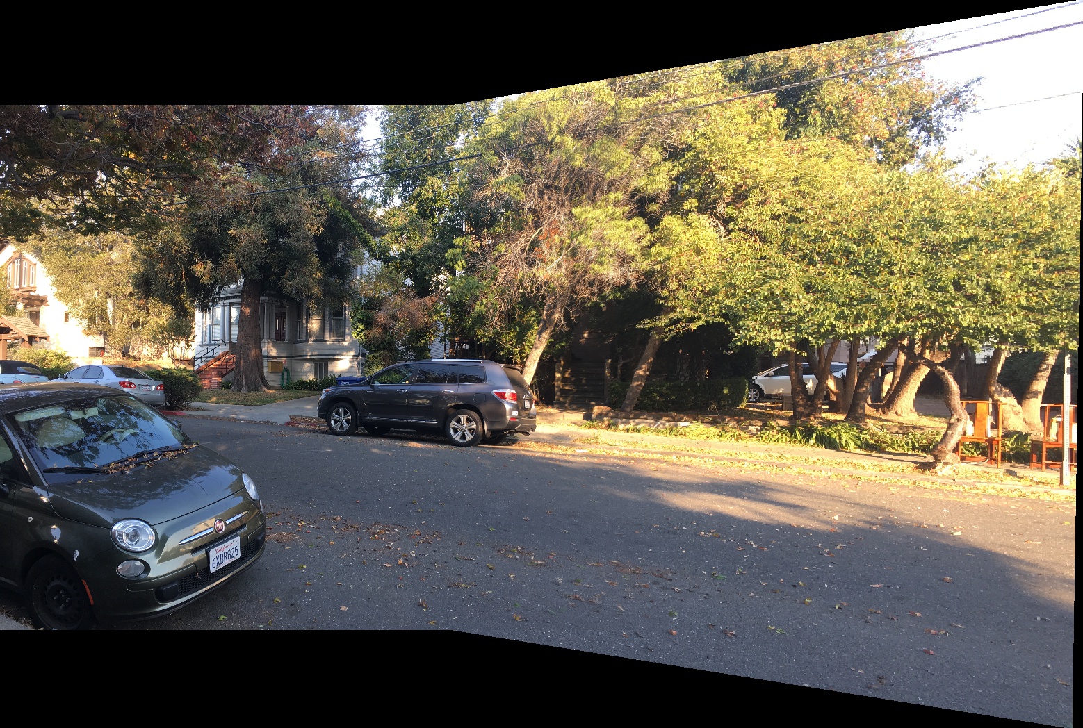
We can compute homographies, which are projective transformations (i.e. arbitrary quadrilateral mappings). These homographies can be used to define which parts of images should look rectangular (rectification) or can be used to stitch panoramas together (to produce image mosaics) by identifying a set of at least four correspondence points between the two images to be stitched. (I found 8 points to work well)
Part 6B
Summary
Manually defining correspondences can be annoying and prone to human error. In this part of the project, we'll develop a method for automatically detecting features and finding good correspondences automatically.
First, we'll use Harris Point Detection (min_dist=5, sigma=12, edge_discard=100) to find strong corners in both our images, like below:


Then, we take all of these corners and run ANMS (in theory -- I just took all of the corners and did not complete the ANMS section).
We take the points that we have so far and extract patches around them. We downsample these patches in order to do low-frequency comparisons (which should guard against small changes in camera angle, etc). Afterwards, we want to try to match these patches. We are assuming that both images will share some strong corners, and so we run an O(N^2) algorithm that compares each patch on the left with all patches on the right and remembers the "best" one. We define the best correspondence between two patches as minimizing the 2-d distance between the patches, i.e. finding which two patches look most similar. For each patch in the left image, we find the two best matching patches in the right image. We can then take the ratio of their scores (best_match / second_best_match) and compare that to our Lowe threshold (I used 0.8). If our ratio is less than that, we can say with higher confidence that the best match actually found a valid patch match. (if the ratio is higher, then maybe that feature is not distinctive enough to justify a match).
After that, we're left with a set of correspondences that looks something like:


Now, we want to find which of these points we should use to compute our homography. We iteratively do the following (I iterated ~4000 times):
- Randomly select 4 left-right corresponding corners.
- Check that have not already tried this permutation of corners. If we have, repeat the above step.
- Compute a homography with these 4 points.
- Apply this homography to all points on the left, and check if the positional SSD between the transformed point and the expected point in the other image is within some epsilon distance.
- Count the number of times the above statement is true.
- Return the homography for which the above statement had the highest count.