


CS 194-26 Project 6
Borong Zhang cs194-26-agb
Overview of the Part A
In this part, we use projective transformation to stitch images together. By choosing corresponding points, we are able to create image mosaics similar to a panorama.
Stitching Photo Mosaics
Image Rectification
Mosaic
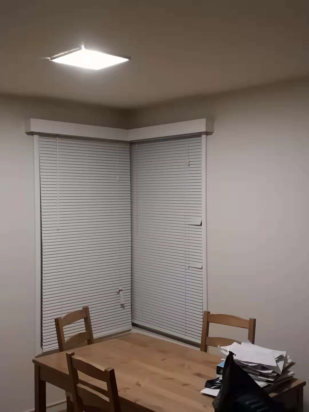
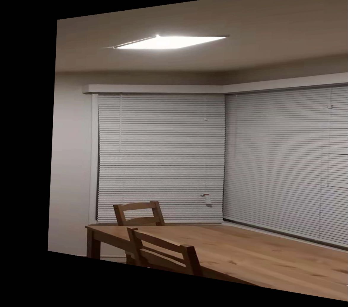
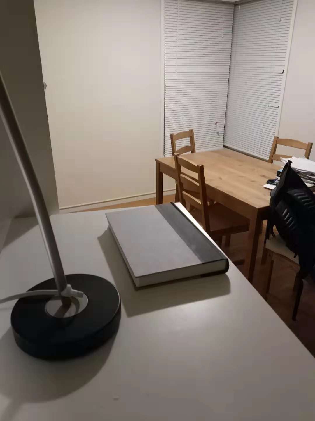
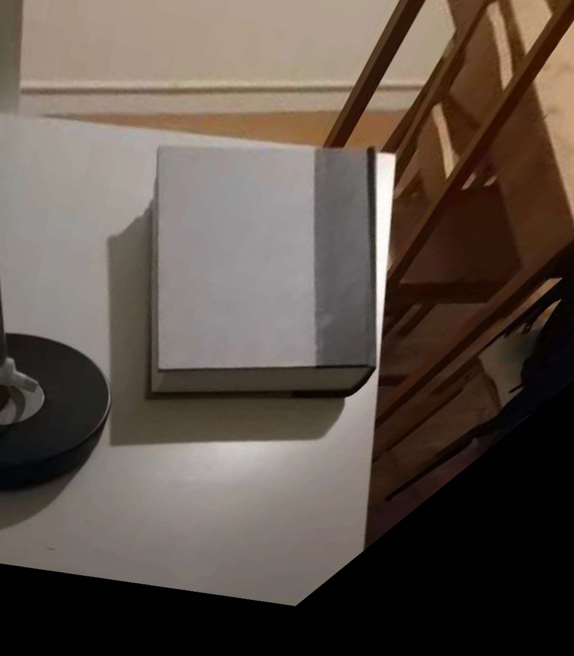
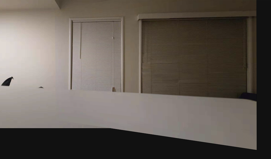
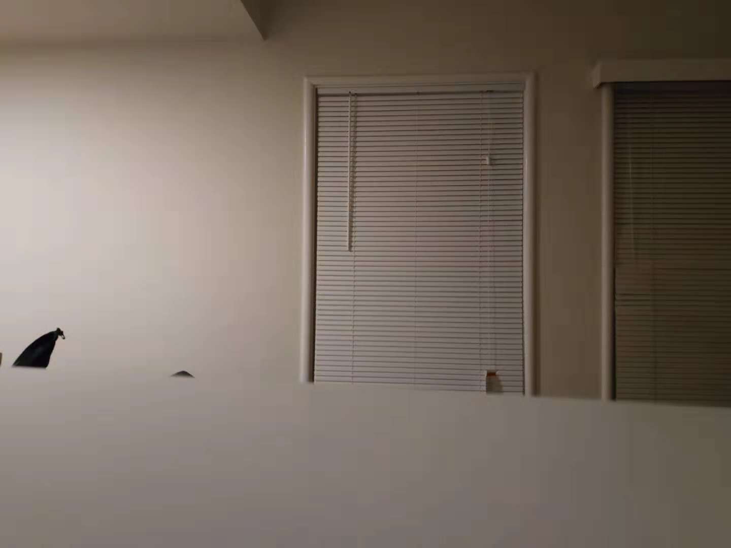
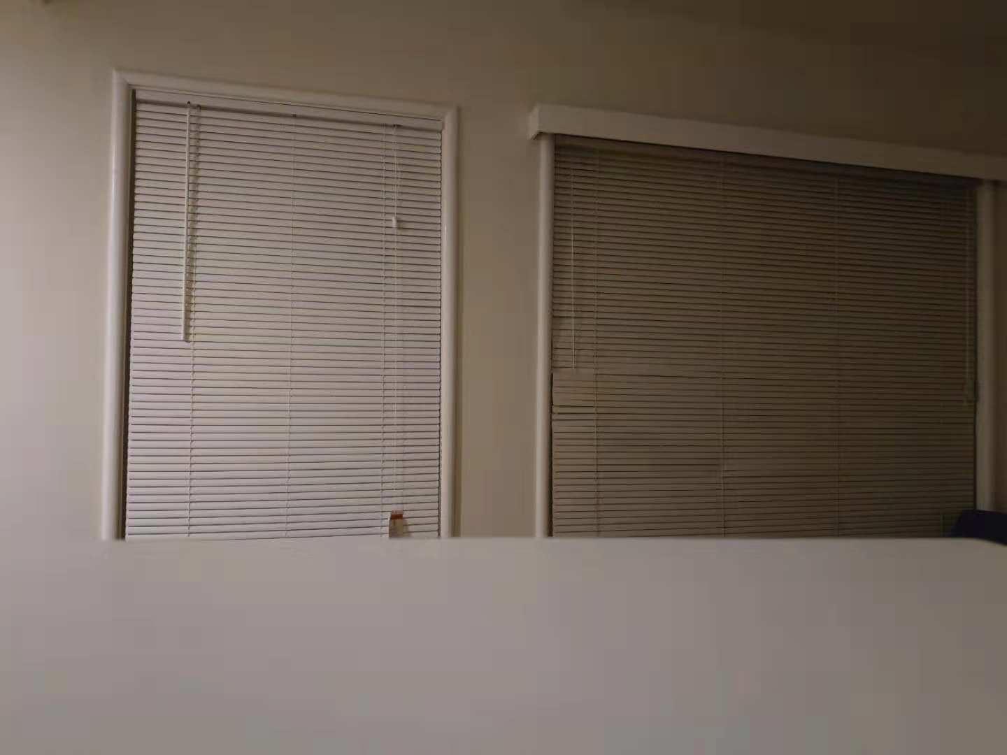
In this part, I warp images so that the plane is frontal-parallel (rectified). In the first example, I rectified the window and in the second example, I rectified the book.
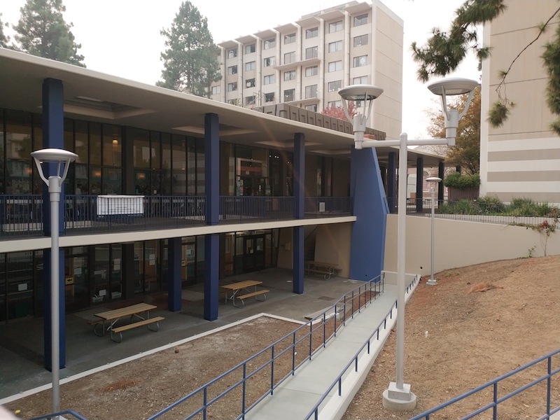
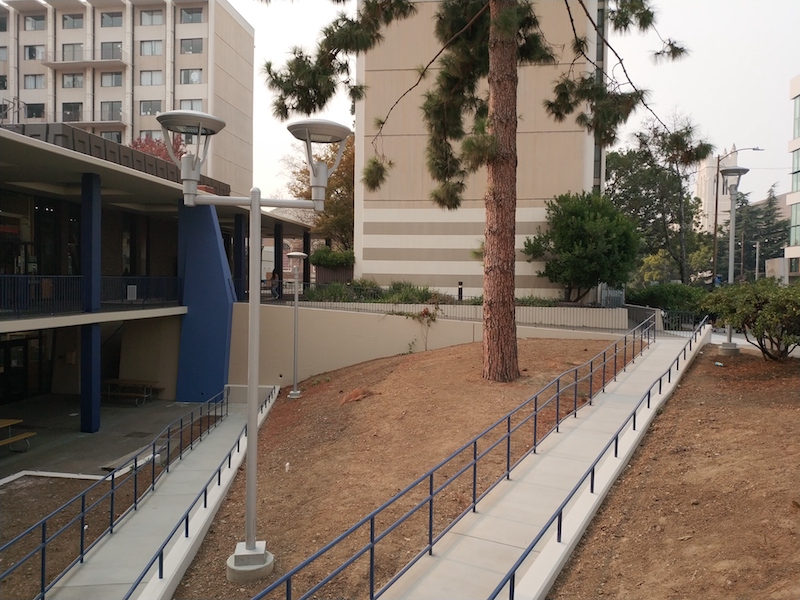
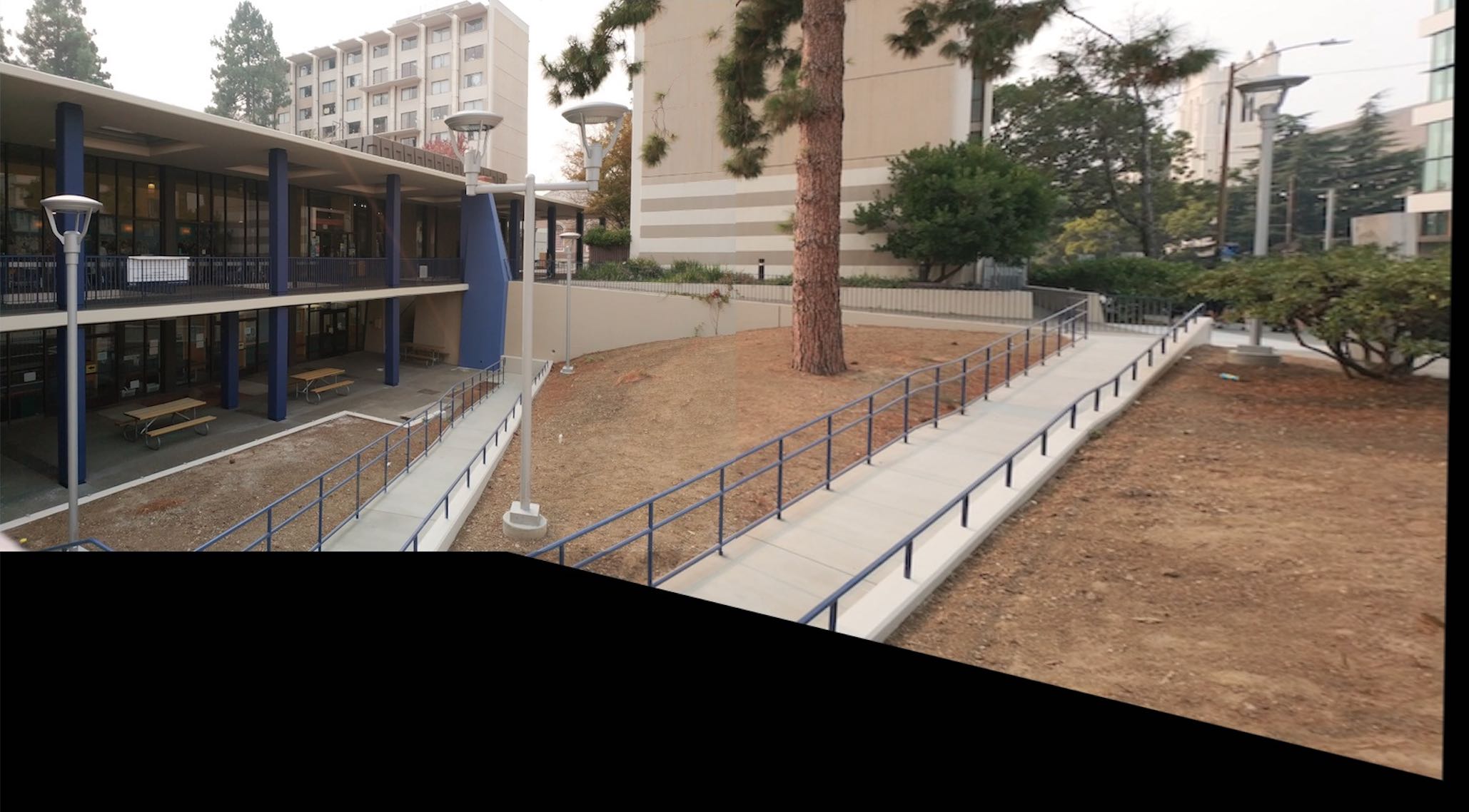
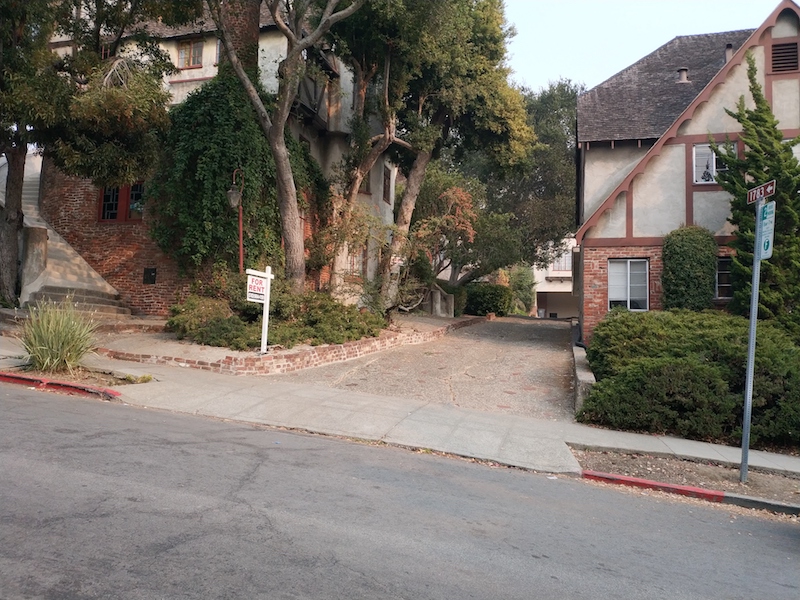
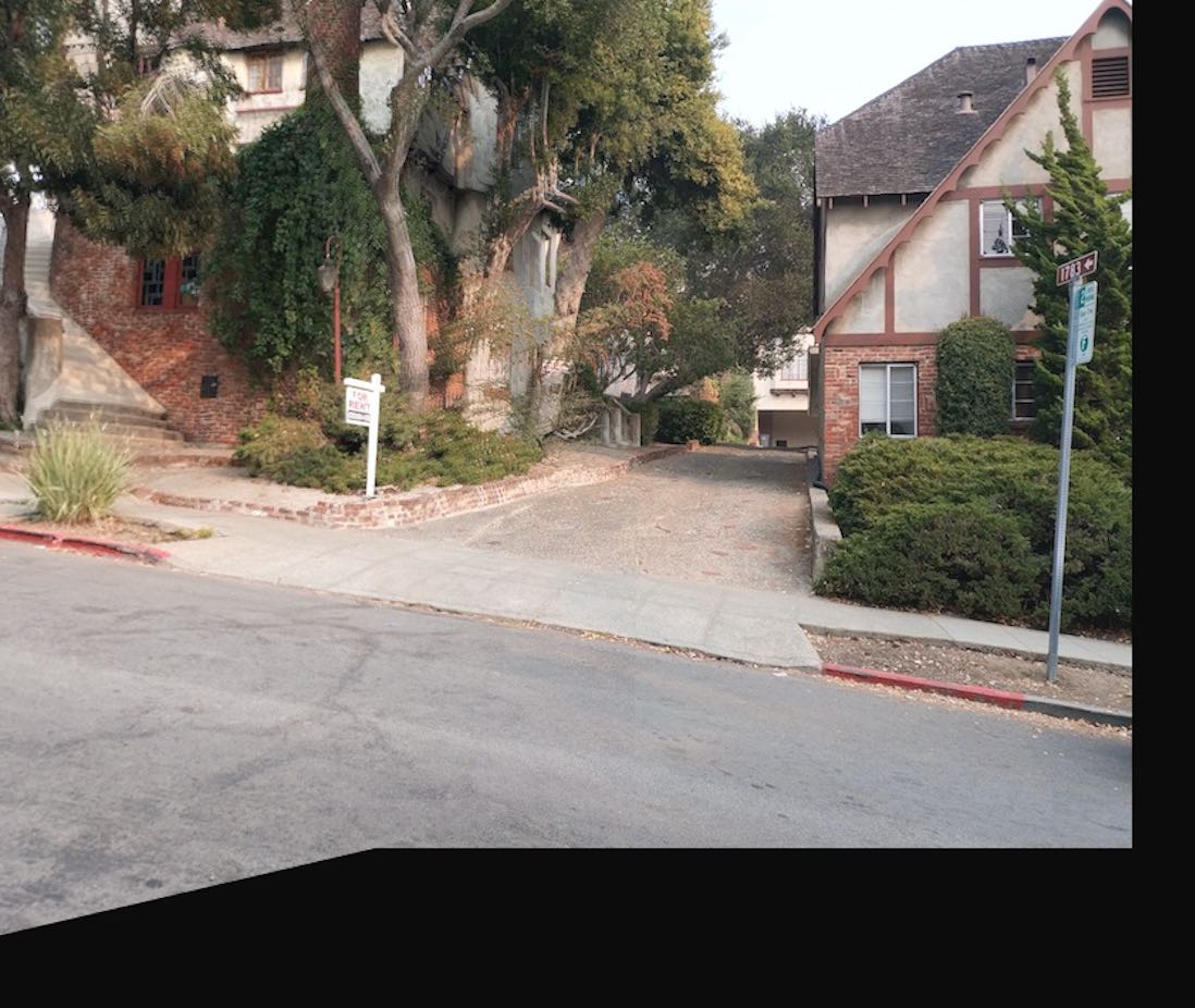
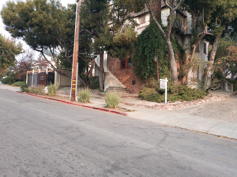
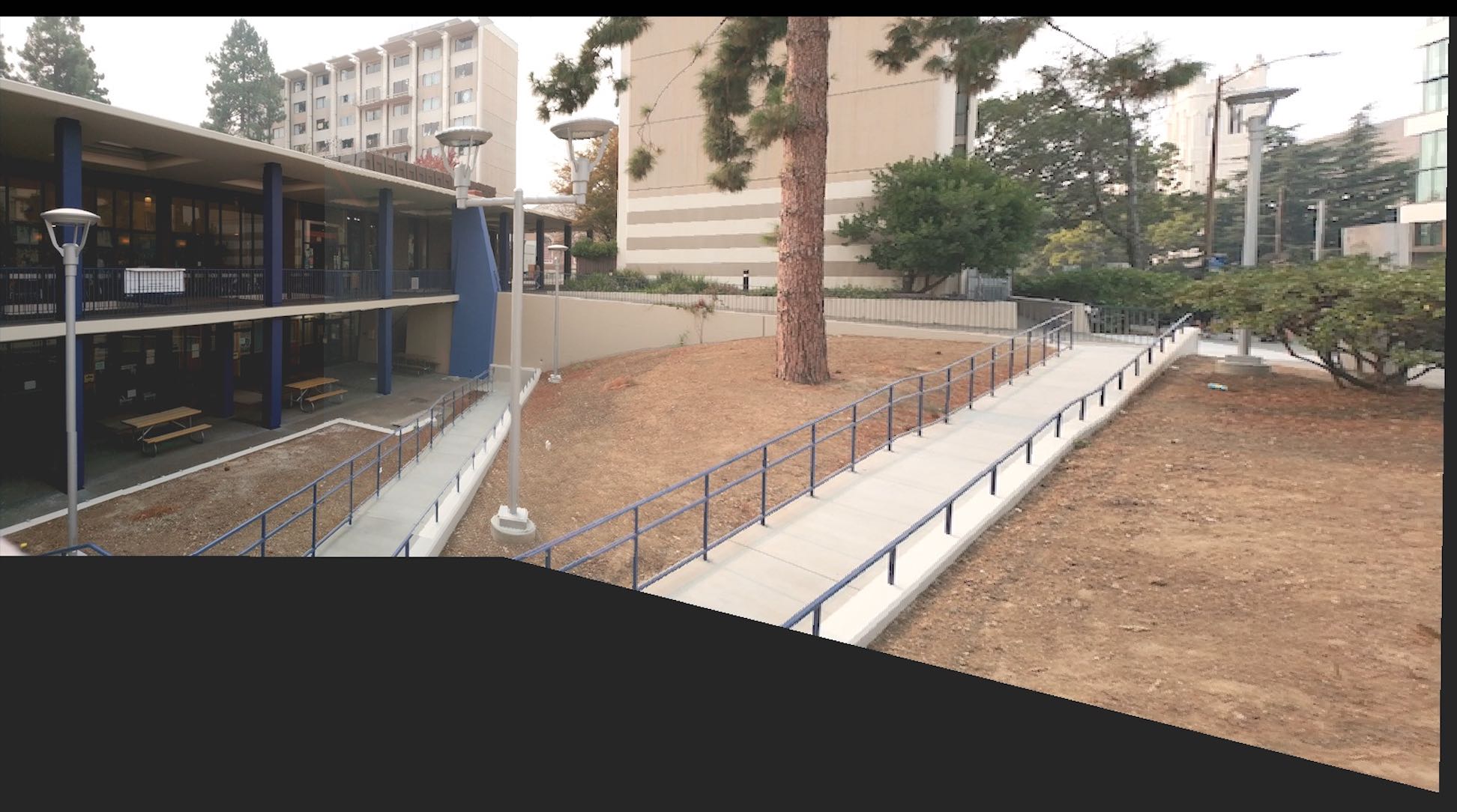
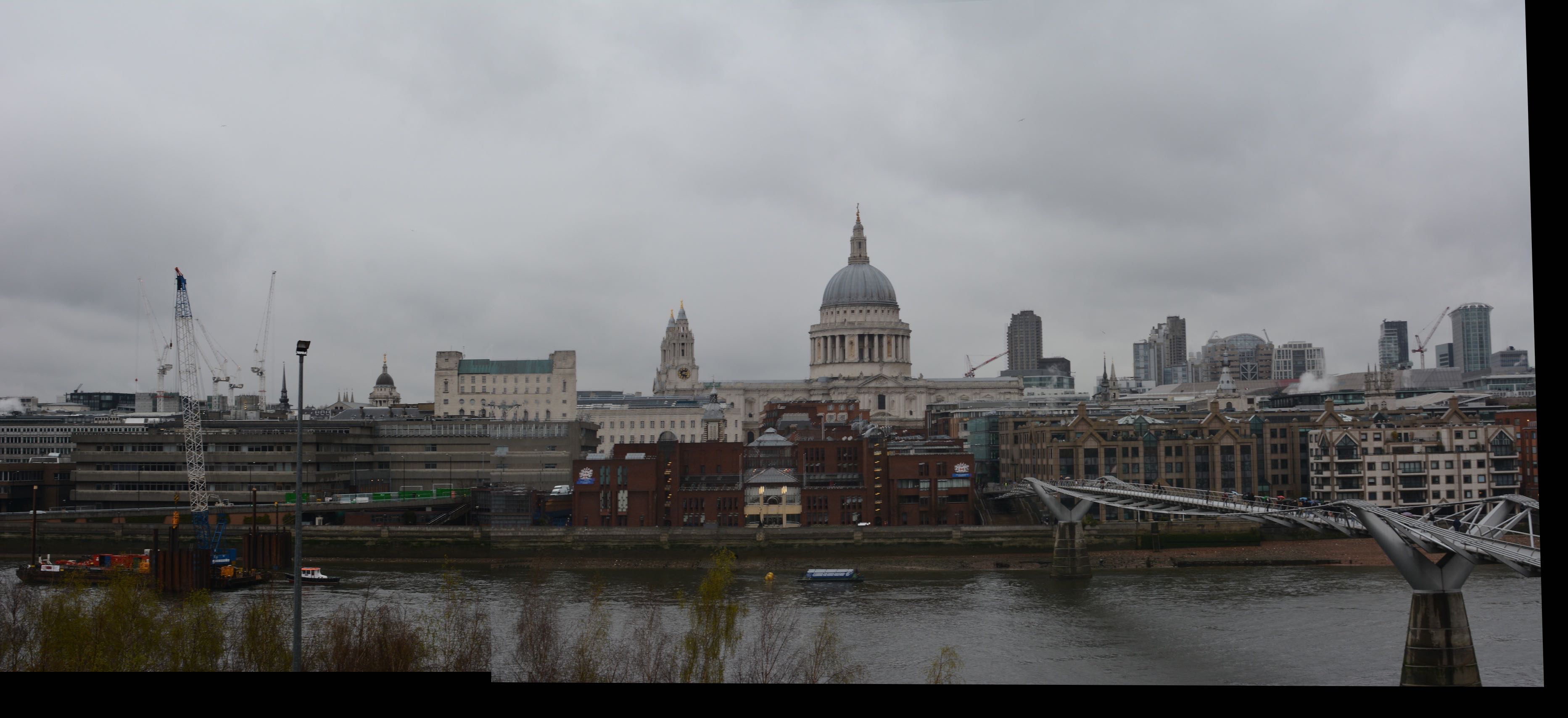
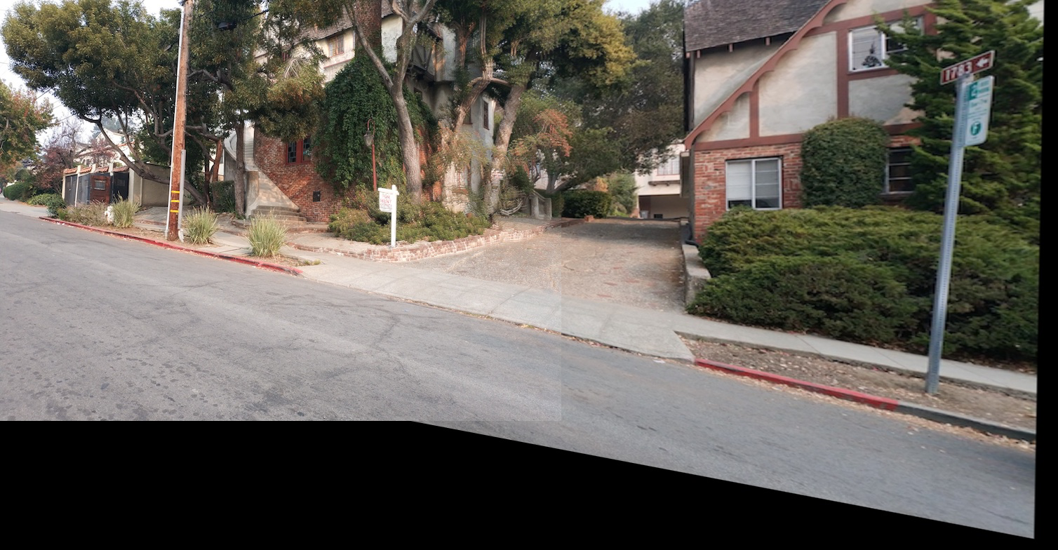
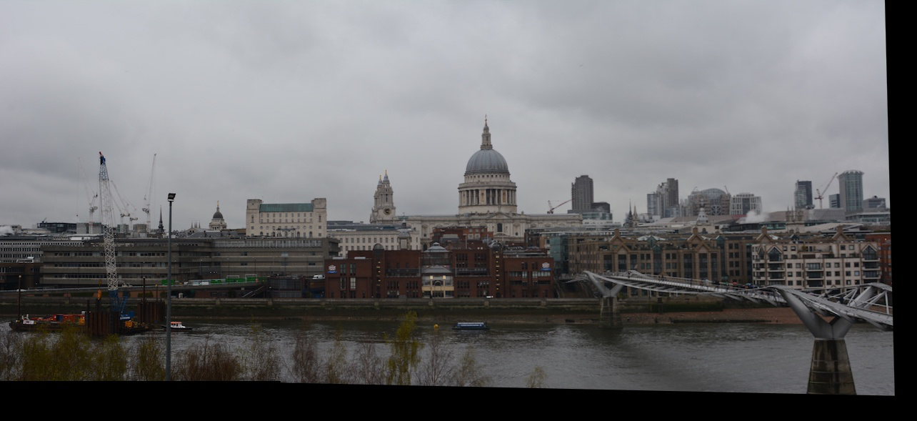
In this part, we first find corresponding points between two images and then stitch them together by projective tranformation to create mosaic.
What I learned
1. Picking points is tedious.
2. I need to get a digital camera!
3. Homograph is really cool.
4. Linear algebra is powerful.
Overview of the Part B
In this part, we used slightly-simplified versions of the algorithms described in the paper Multi-Image Matching using Multi-Scale Oriented Patches to automatically detect and match corresponding points between two images. These correspondences are then used to stitch the images together to form a mosaic, as in the previous part.
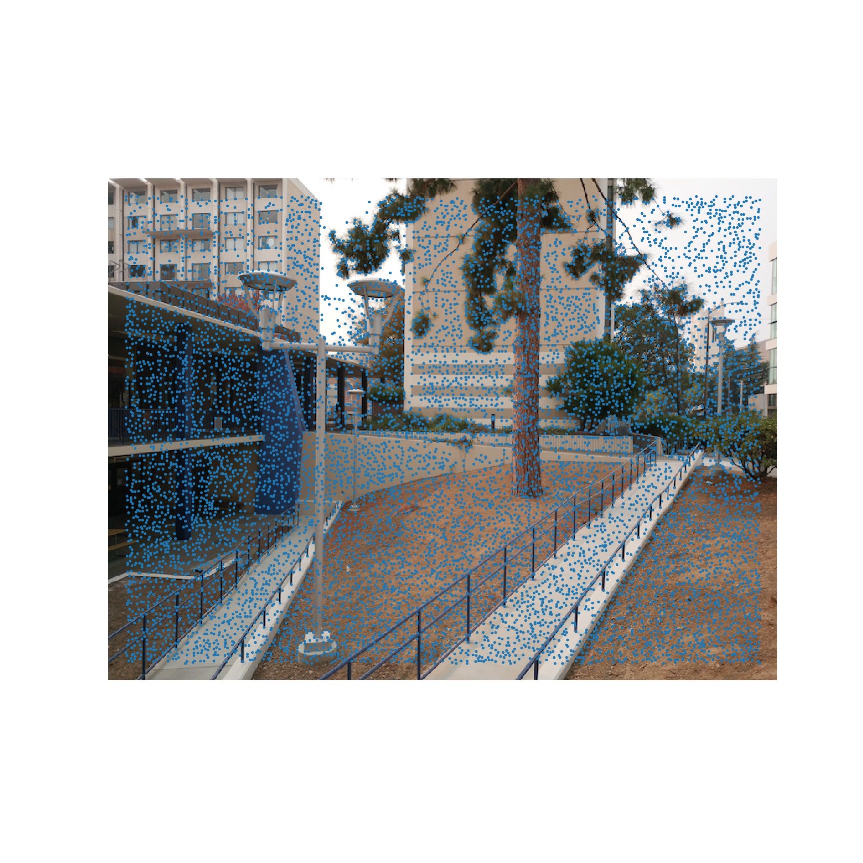
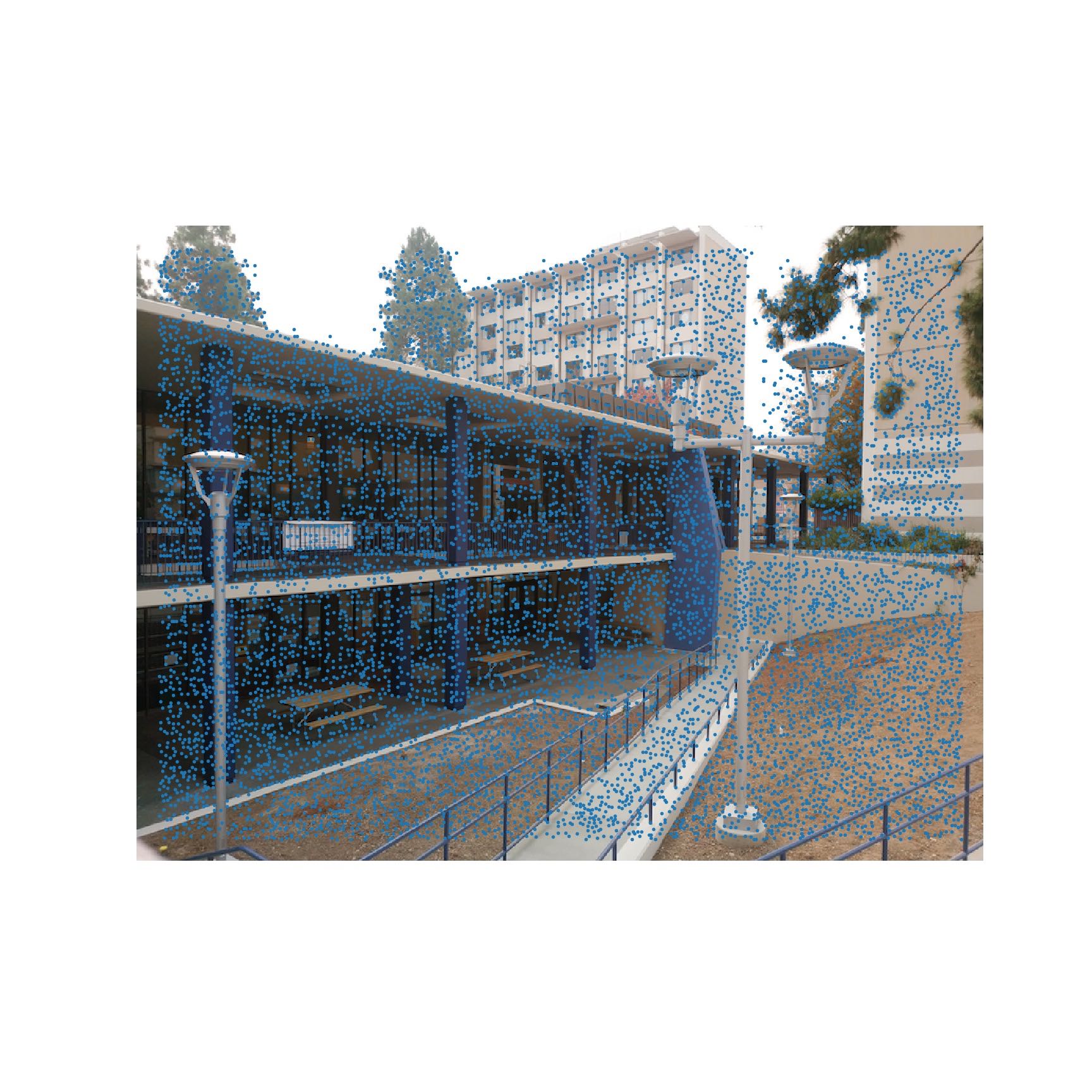
Harris Interest Point Detector
Adaptive Non-Maximal Suppression
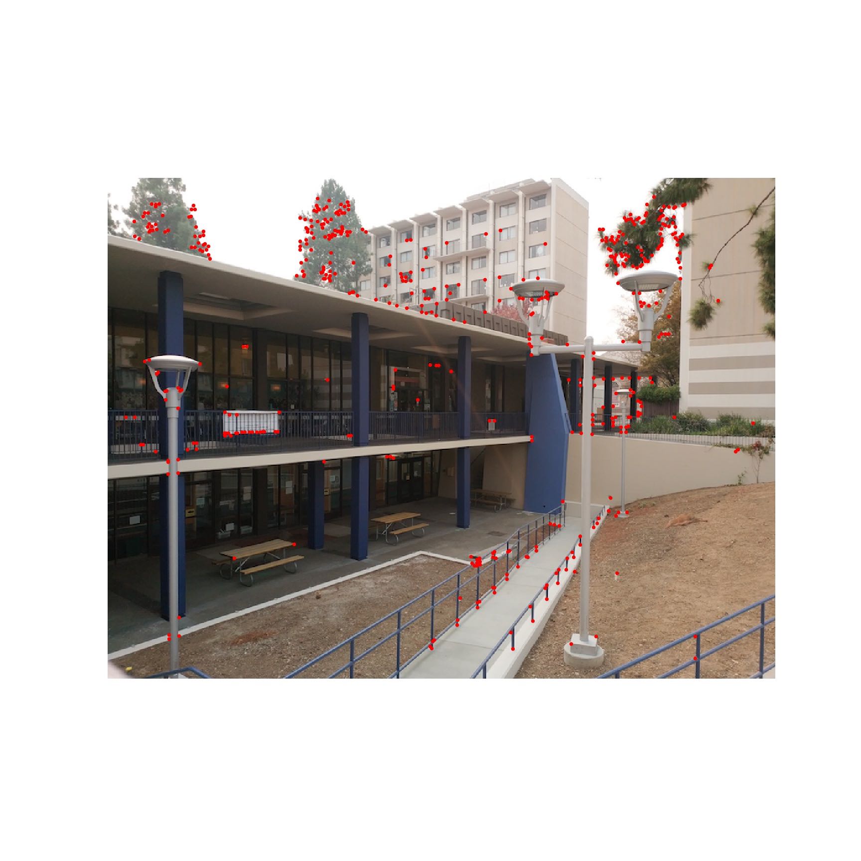
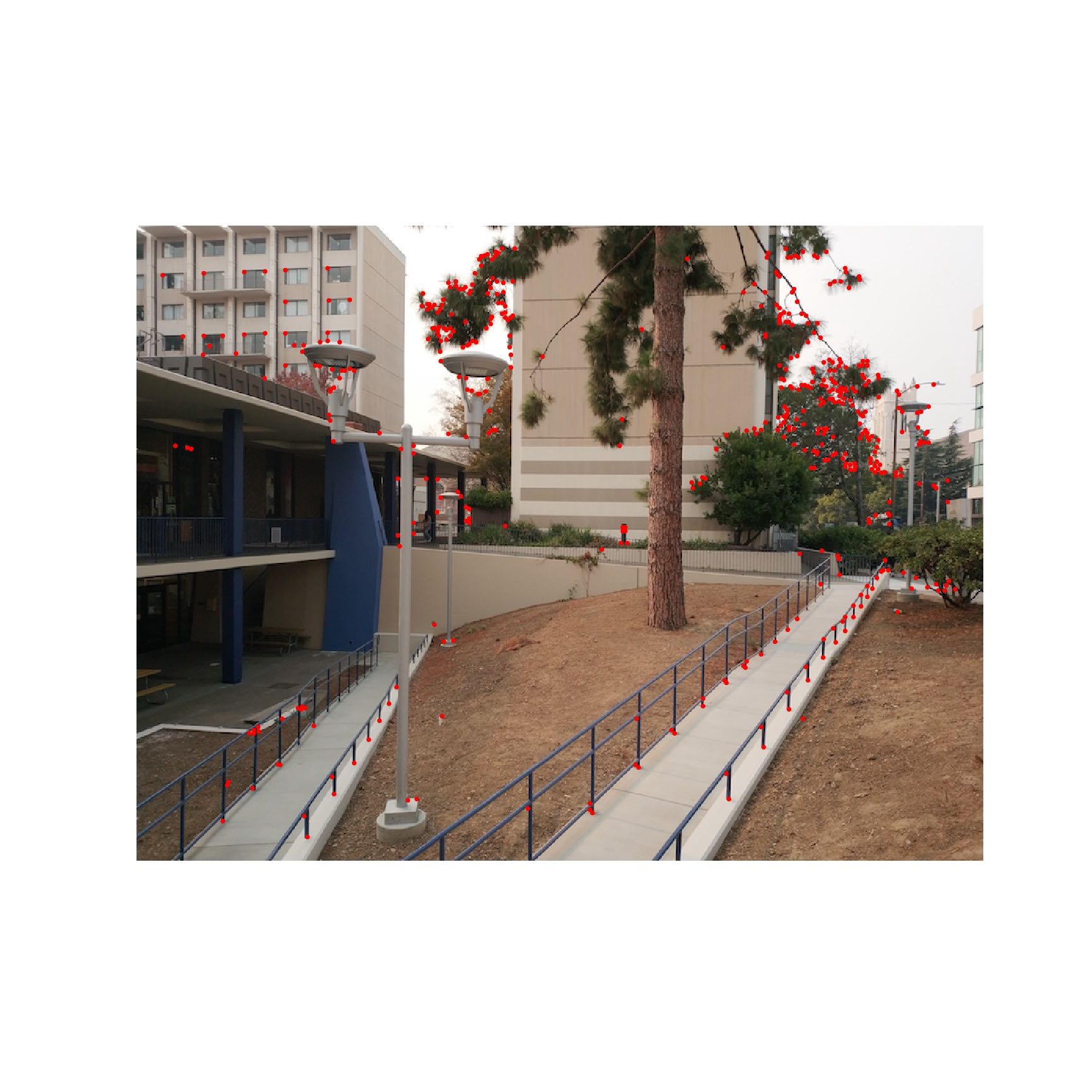
Using the provided code for finding Harris points of an image, we can find places that look like corners. It does this by evaluating product and sum of eigenvalues of the matrix constructed by imge derivatives. Product and sum of eigenvalues of a matrix are equal to determinant and trace of it.
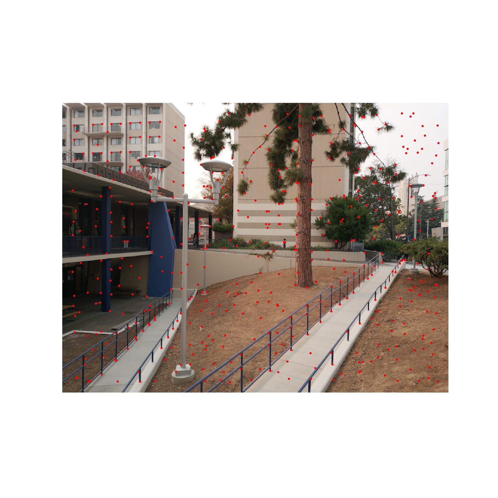
Since there are too many harris points, we need to filter out some of them. Firstly, we pick top 500 points with highest values.
Feature Descriptor Extraction and Feature Matching
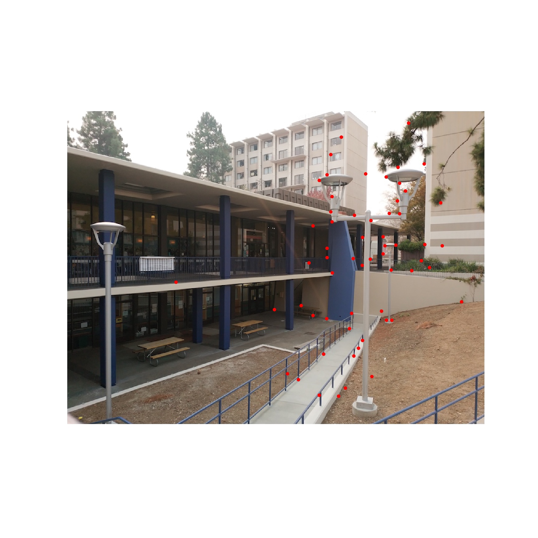
In this part, we use our interest points as feature descriptors. From each corner, we extract a feature descriptor - a 40x40 region around the corner, resize it down to an 8 x 8. Then, using the feature descriptors found above, we can find matches. By thresholding the interest points by their Lowe ratio, we get feature matches between our source images:
RANSAC and Computing Homography
Even after computing matching feature points, there was still the case of possible outlier which would mess up homography computation and warping. Thus, we used RANSAC to get rid of outliers. In RANSAC we select 4 random points from the matching point list, compute the homography, and apply the transformation to all of the feature points. The transformed points that were within 1 pixel of where they should have been in the second image, we kept as the inlier set. We repeated this process 10,000 times and kept a record of the largest inlier set. After the iterations, we used this inliner set to compute our final homography that we used to warp and blend our images. The rest of the image warping and blending followed suit to the steps above in the manual mosaic blending.
Below we show the inliner set chosen after RANSAC and the final blending results.
Results
Manual labelling
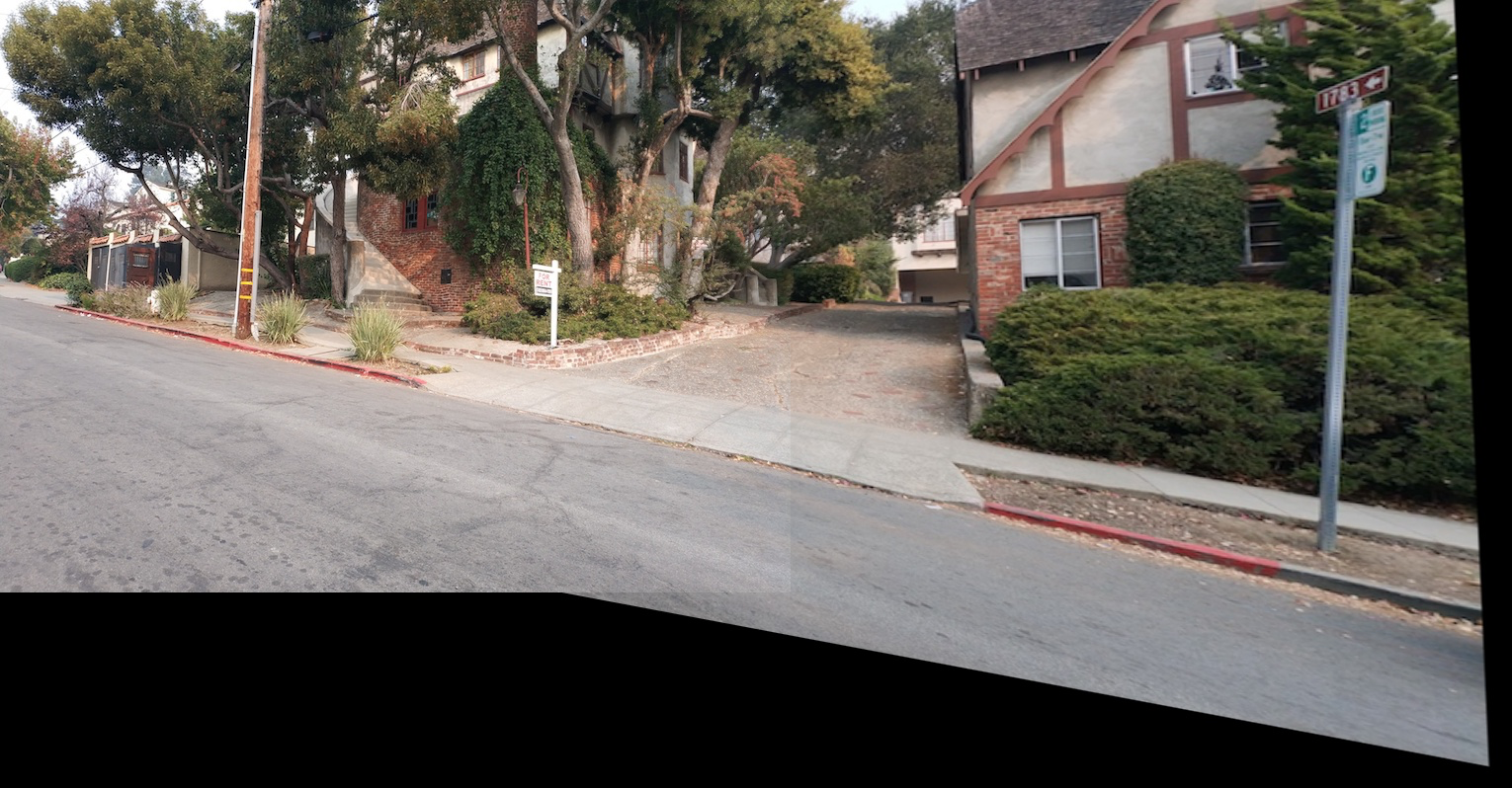
Automatic labelling
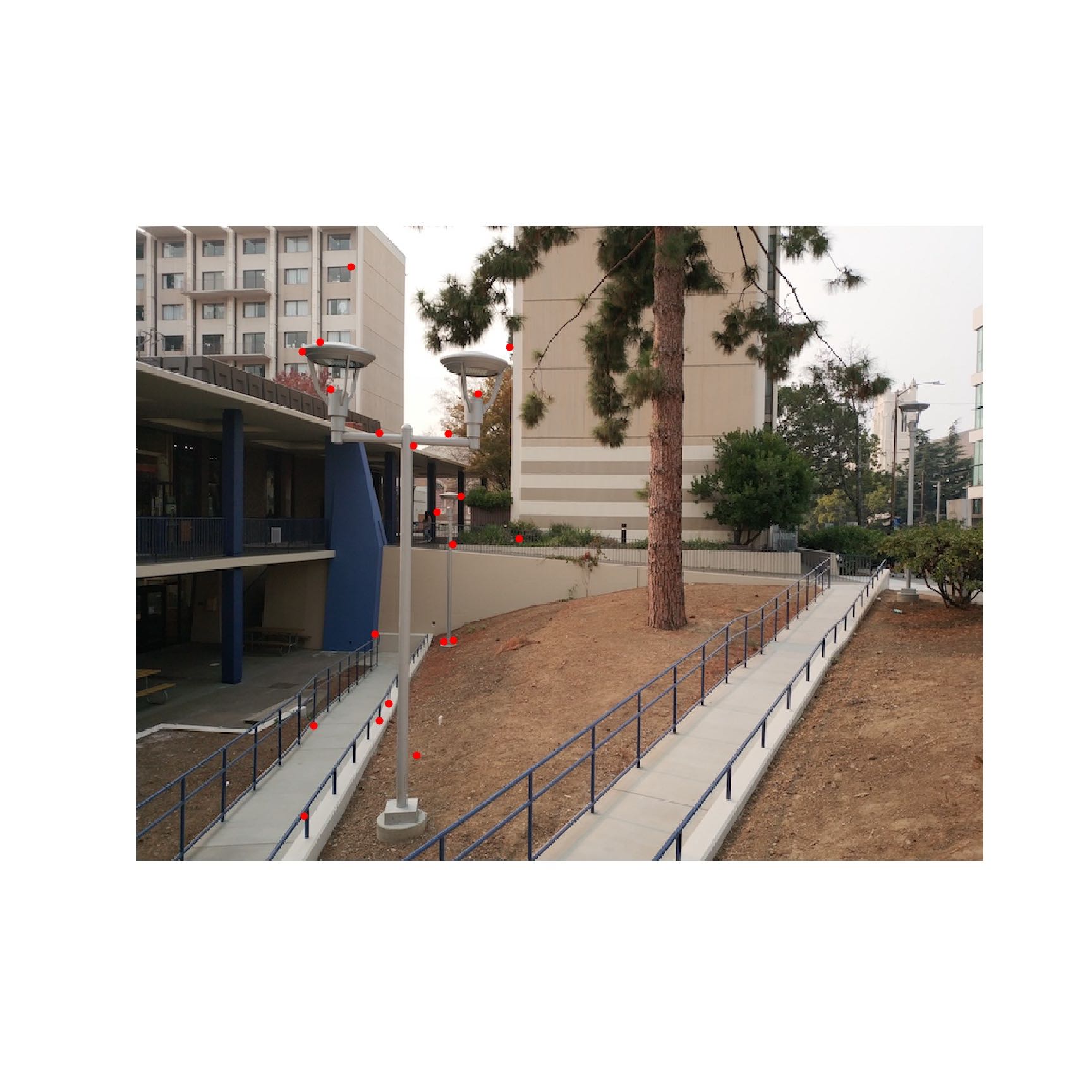
However, using the method above, we get clusters of points, which is not optimal because later we want our matched points to be more separate. Then, as describe in the paper, for each point, we find the minimum radius to the next point such that the corner response for the existing point is less than some constant multiplied by the response for the other point. We let the constant be 0.9 and take the top 500 points:
Manual labelling
Automatic labelling
Manual labelling
Automatic labelling
Clearly, for all three examples, manually labelled results are a little bit more blurred then automatically labelled results. It's partly because I only use 8 manually labelled points.
What have you learned?
The most interesting thing I have learned is how robust automatic feature matching was. It's fast and always produces better results then manually labeled results. Also, I learned so much by debugging and correcting methods. It's just astonishing that a seemingly simple project can have so many details to be taken care of.