Part A: Image Warping and Mosaicking
In the first half of the project, our goal is to produce mosaics generated from multiple images. To achieve this, we must set up correspondence points between images, define and apply projective warps, and composite.
Shooting Photos
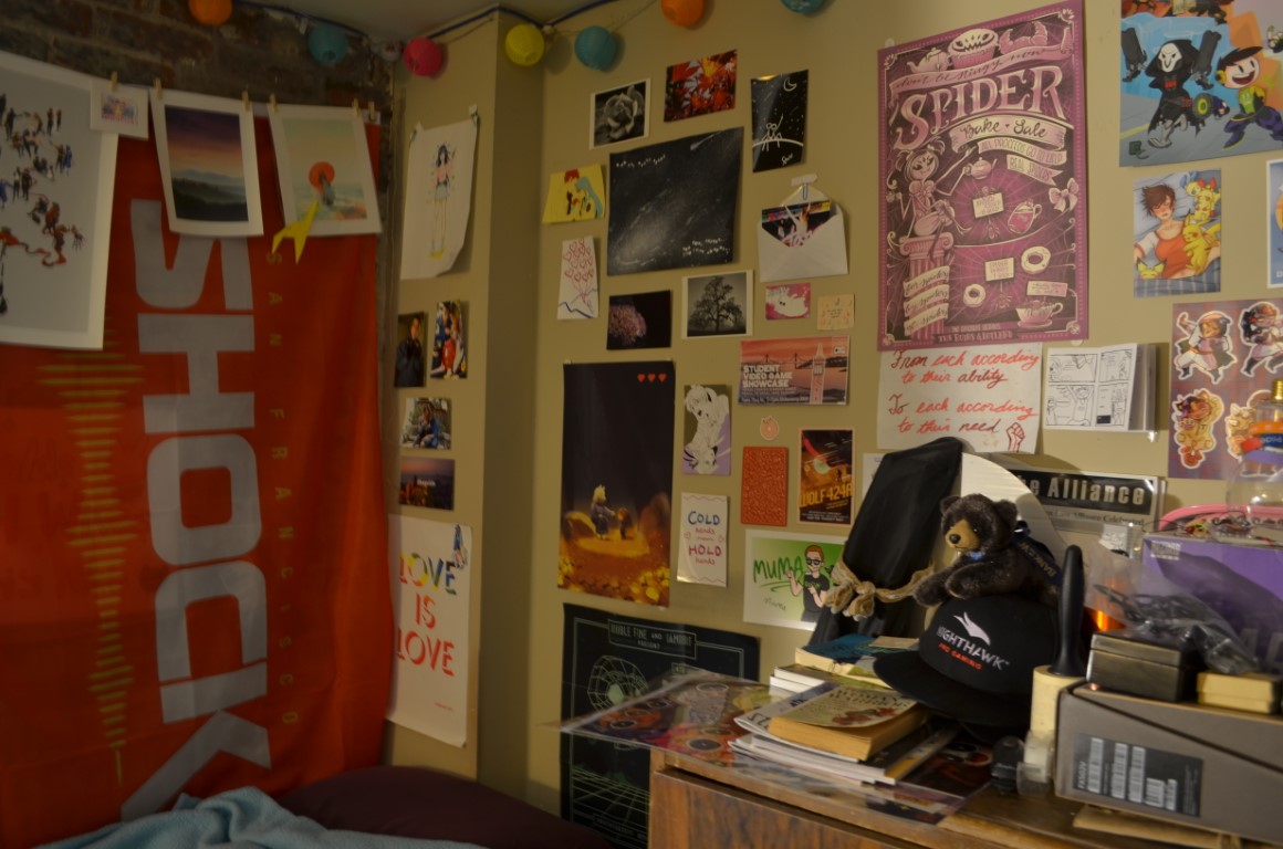
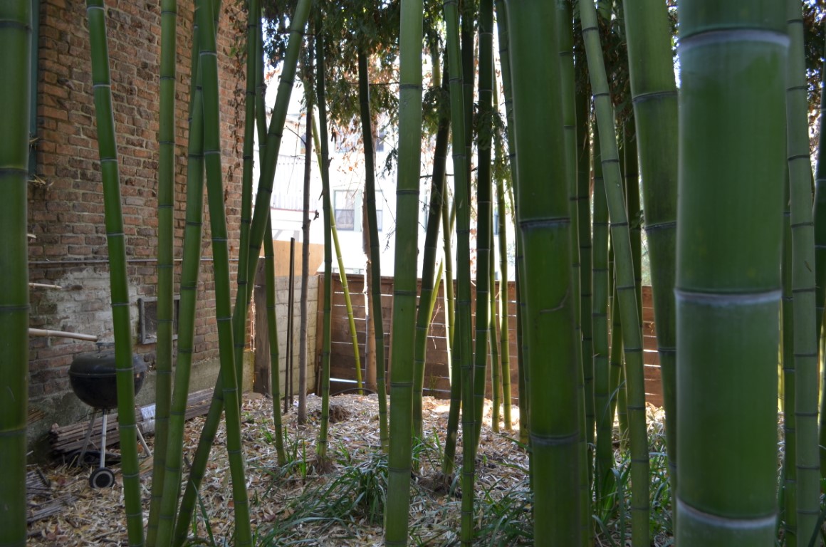
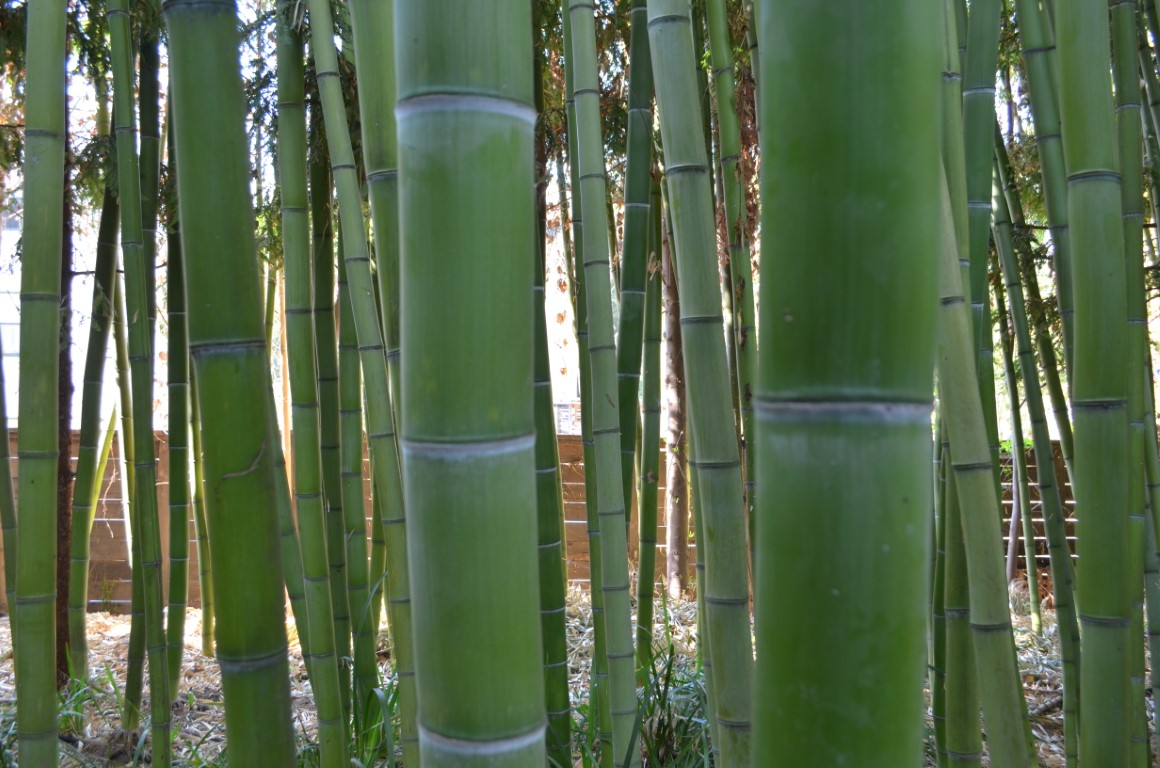
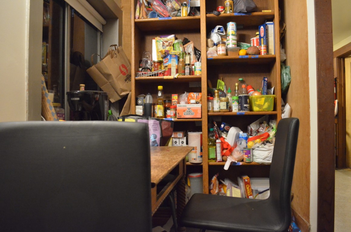
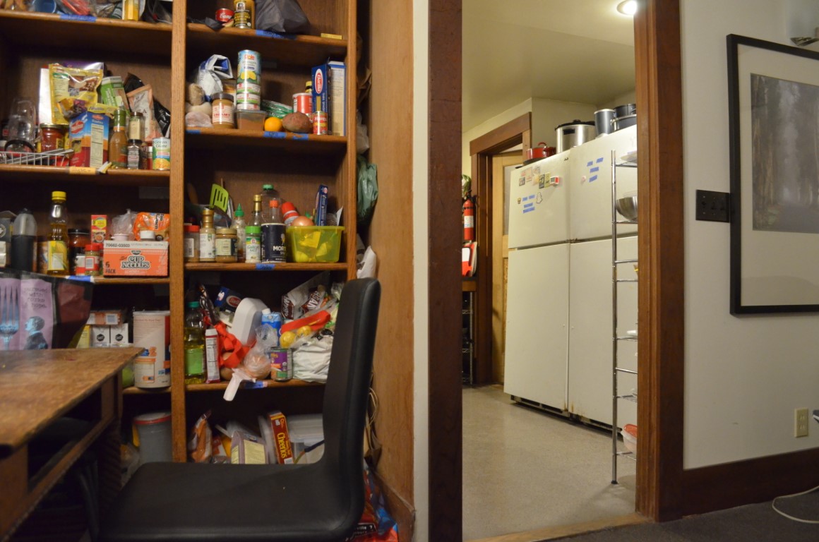
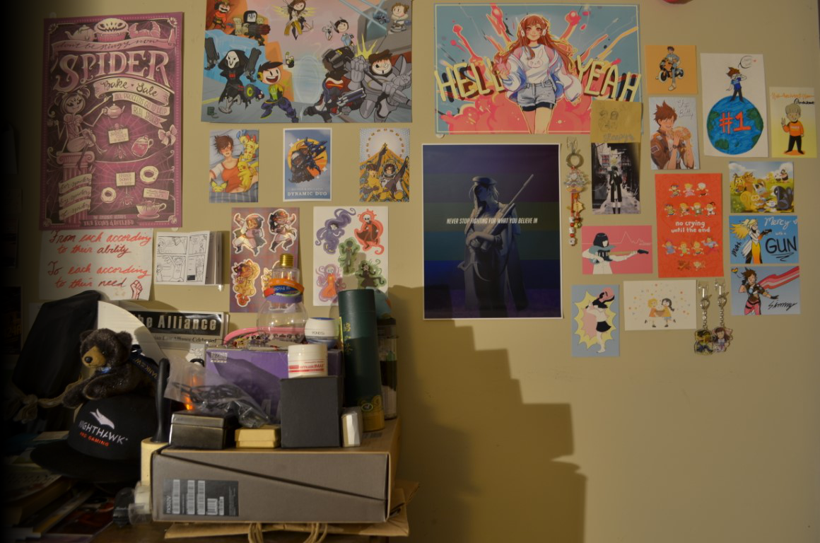
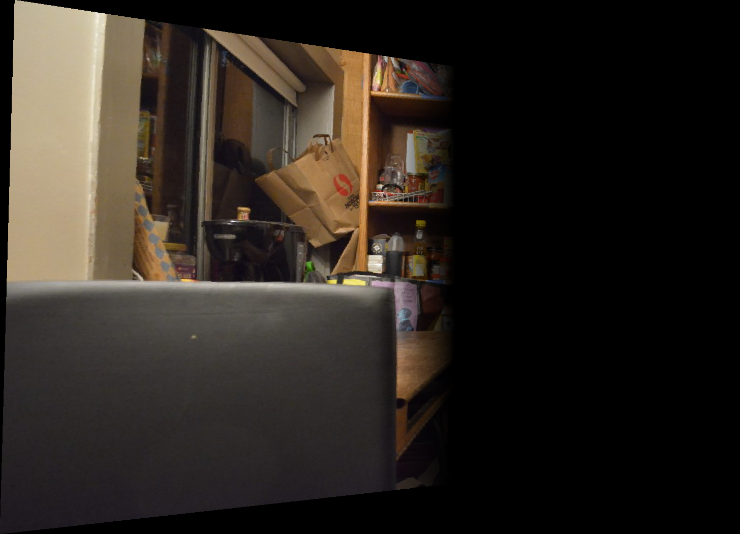
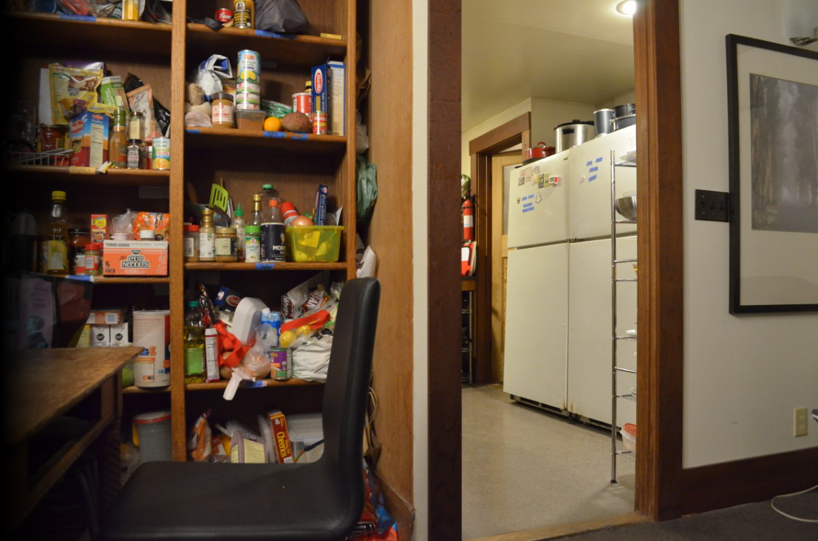
In order to generate mosaics, we must first take several photos. One way we can do this is by taking pictures from the same location, but rotating the camera to capture overlapping fields of view. We captured the three following sets of images.

Recovering Homographies
Before we can warp one image to align with another, we must first determine
the parameters defining the transformation between the two images. That is,
we must find the parameters of H in p' = H * p,
where H is 3x3 with 8 degrees of freedom (the ninth being a scaling factor we set to 1).
We can find these parameters by solving a least squares problem generated
from n point correspondences between a pair of images. At
minimum, we need n=4 pairs of points, but this would result in
a noisy/unstable homography; thus, my image pairs typically use 8
correspondence pairs defined manually using Python's ginput.
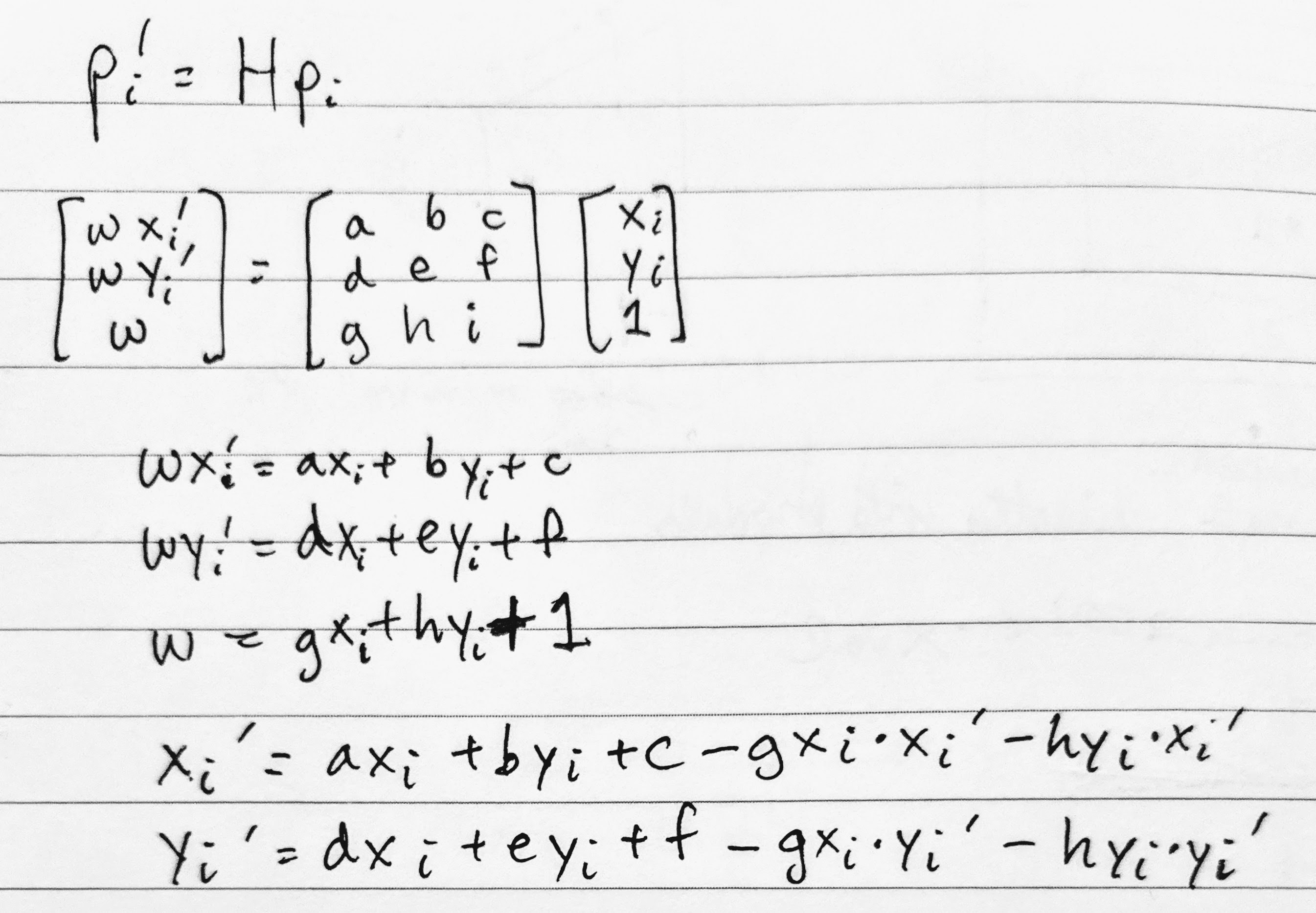
The following is the derivation of the least squares setup. We
begin with the relationship between the ith point (p_i)
and its transformed counterpart (p_i'). Performing the
matrix multiplication, we get the three equations in the middle block.
Substituting w = g * x_i + h * y_i + 1 into the other two
equations, we get the last two equations that we can use in our setup for
every pair of points. That is, we add x_i' and y_i'
to b and the coefficients on the right-hand side to
A.
Note that our h in A * h = b is
flattened from 3x3 to 8x1 for the 8 unknown degrees of freedom (p_i'
is merely the scaling factor).
Warping Images and Rectification
Now that we know the parameters of the homography, we now have the transformation matrix we can apply to all of the points of an image in order to warp it. What we can do here is first forward warp the corners of the original image so we can determine the bounding box of the new image. Based on this bounding box, we can iterate over it and inverse warp back to the original image to sample the pixel colors. If a pixel in the warped image's bounding box maps to a pixel in the original image, we copy the original image's pixel colors to this pixel.
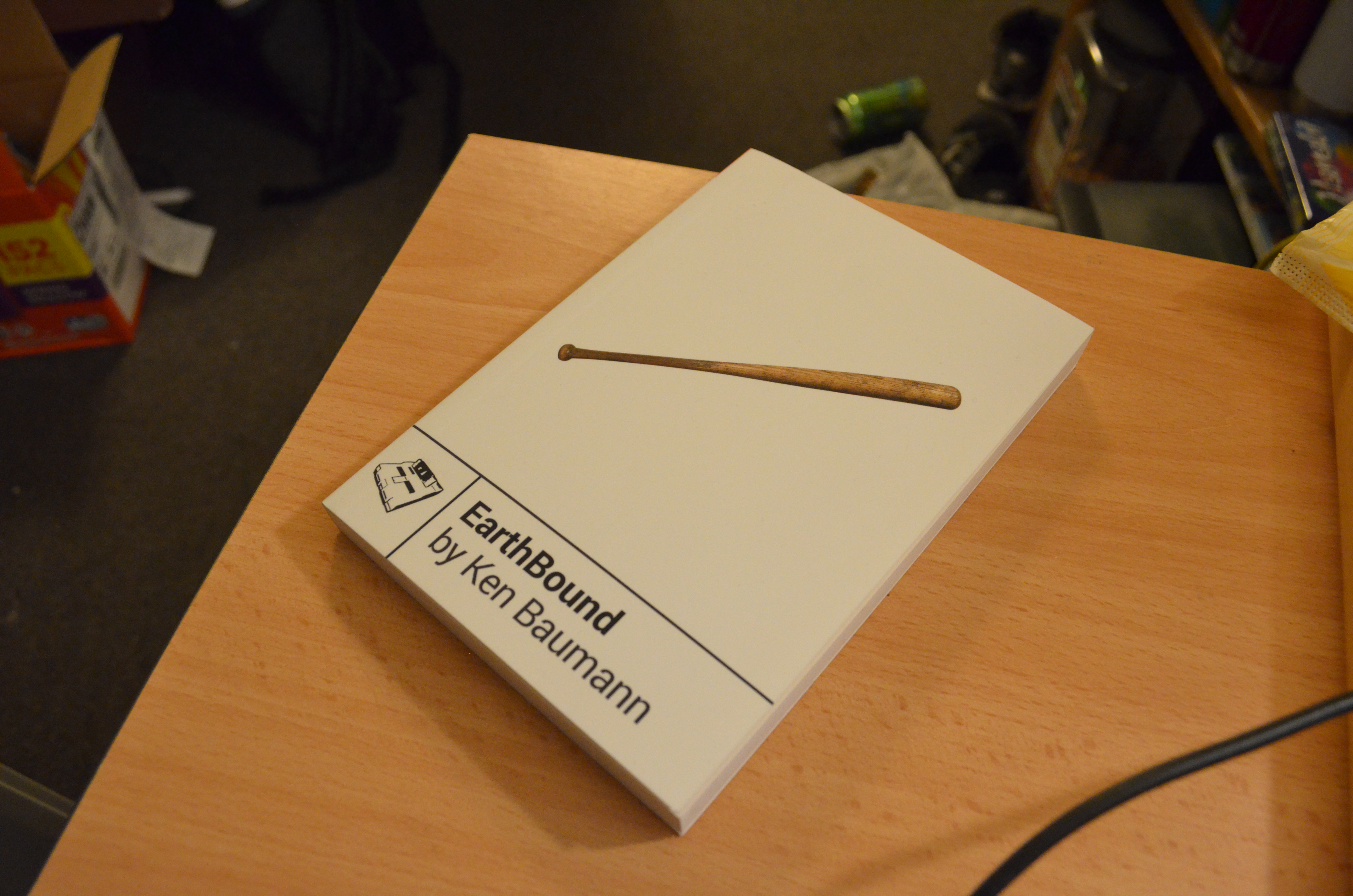
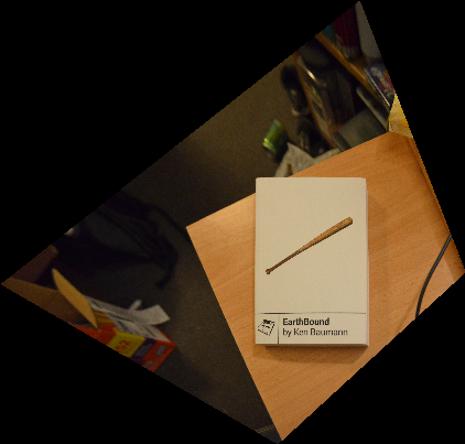
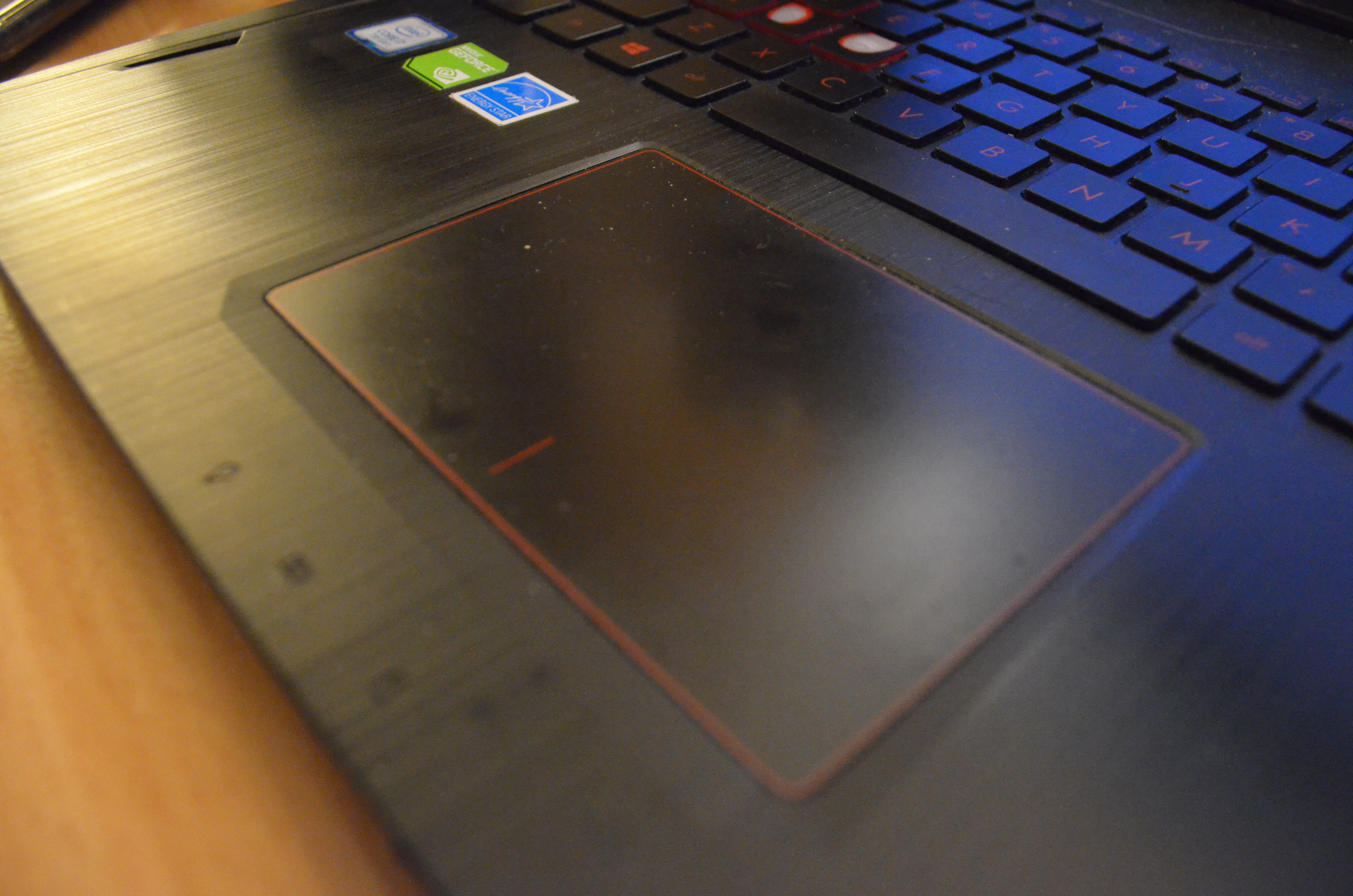
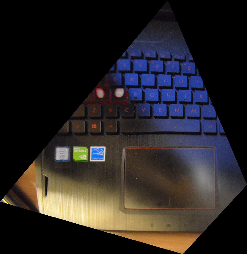
We can test out our image warping for the application of rectifying images. We can rectifying images simply by selecting four corners in the original image and defining the correspondences to match a rectangle's four corners. Below are the results of rectifying a book and a trackpad:
Blending Images into Mosaics
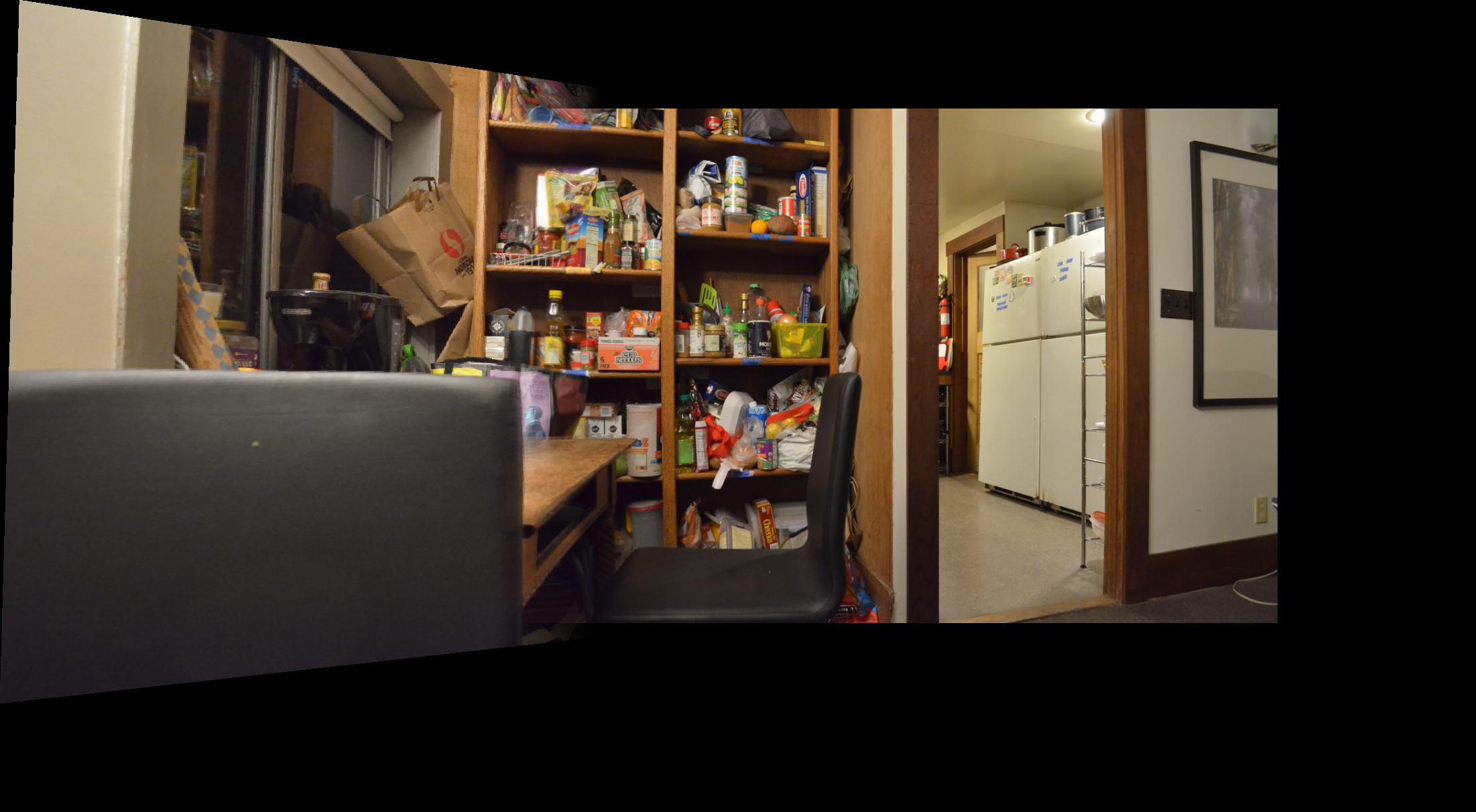
Once we are able to warp images from one projection to another - i.e. from the perspective of one image to the perspective of another via their correspondence points - we are able to create our mosaics. All we have to do now is implement some sort of blending to reduce the obvious edge that would result from simply overlaying one image on top of the other. We can achieve this with simple alpha blending, masking both images and then compositing them into a final image.


What I've Learned from Part A
One thing I've learned - or perhaps the word is "internalized" - is just how our brain deceives us. Things that we perceive as being rectangular are actually trapezoids or other parallelograms; rarely are they truly rectilinear. It's just that our brain, over time, has learned to process these images as "rectangles." However, when we perform mosaicking, we cannot take this fact for granted. We have to warp images to be truly rectangular to produce a satisfying result.
Another thing I've learned is that plenty of the concepts we've used in previous projects keep returning. For example, alpha blending from "Fun with Frequences" and object warping from "Face Morphing" have shown up again, which demonstrates that there are indeed fundamental, reusable concepts within the realm of computational photography and computer vision.
Part B: Feature Matching for Autostitching
In Part A, we implemented the warping and stitching necessary to produce a mosaic of multiple images from manually defined correspondence points. In this half of the project, our goal is to generate automatically defined correspondence points instead of choosing points by hand. To achieve this, we follow this paper with a handful of simplifications.
Harris Interest Point Detection
The first step is detecting corners of an image using a Harris Detector. Luckily, this has been given to us in the starter code, and we can see the results of simply running it on our images.
It would seem there are far too many points of interest right now to process efficiently; indeed, many of them are so close to each other that we can most likely prune this information. So let's do that!
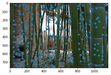
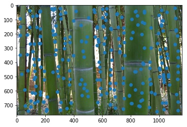
Adaptive Non-Maximal Suppression
Adaptive Non-Maximal Supression (ANMS) will help us reduce what is on the order of 10,000 to 20,000 interest points to, say, just 250 instead. To do this, we iterate over each point/Harris corner we find and find its "radius." We define the radius of each corner as the distance from it to the nearest corner with a Harris corner strength that's at least 10% greater than its own strength. Once we have all the radii, we return the subset of points with the largest radii, i.e. we find the 250 largest radii and choose those points.
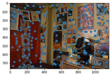
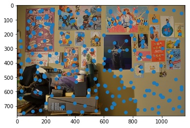
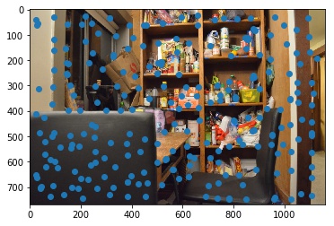
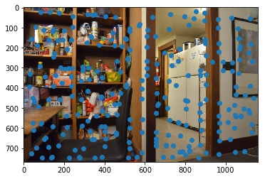
We see the following results. Note that the points are spaced out fairly evenly, covering all sorts of different features in each image and not just clustering around a few of the same features.
Feature Descriptor Extraction
Once we have our smaller set of interest points, we can now produce feature descriptors for each point. We will create a 64-length descriptor vector for each point from an 8x8 patch. This 8x8 patch will be downsampled from a 40x40 window centered around said point.
We also make sure to normalize the vector for bias and gain by subtracting the mean and normalizing to a standard deviation of one. We will then use these descriptors for matching features between images.
Feature Matching
Now we're ready to start matching features. Given two sets of descriptors for two images, we'll calculate the distance between each pair of feature descriptors (specifically, the L2-norm of the difference between vectors).
We will only accept the pair, however, if the ratio between
the nearest neighbor (1-NN)'s distance and the second nearest neighbor (2-NN)'s
distance is less than a threshold of 0.6. That is, we only accept
the pair if dist_{1-NN} / dist_{2-NN} < 0.6. The idea that
if both the nearest neighbor and the second nearest neighbor are of a similar
distance to the current point, then it's likely that the pair is inaccurate
because there should be a clear difference between the two neighbors.
After this step, we see the following pairs of points. The code for this visualization was helpfully provided by Ajay Ramesh on Piazza, as noted in the Acknowledgements section.
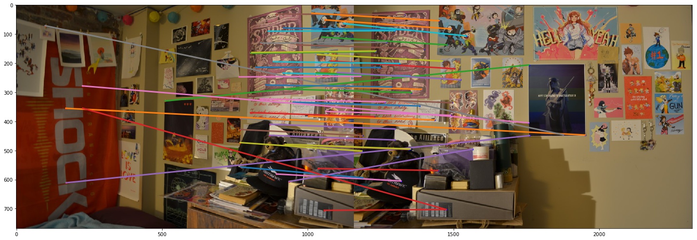
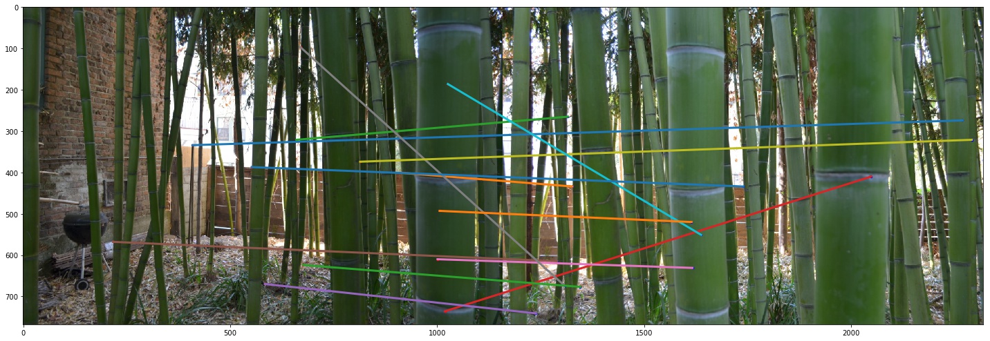
Note, however, that we see a lot of invalid pairs being matched together. That is, some lines are drawn between two points that clearly do not represent the same objects/features. However, we can prune many of these questionable pairs in the next step.
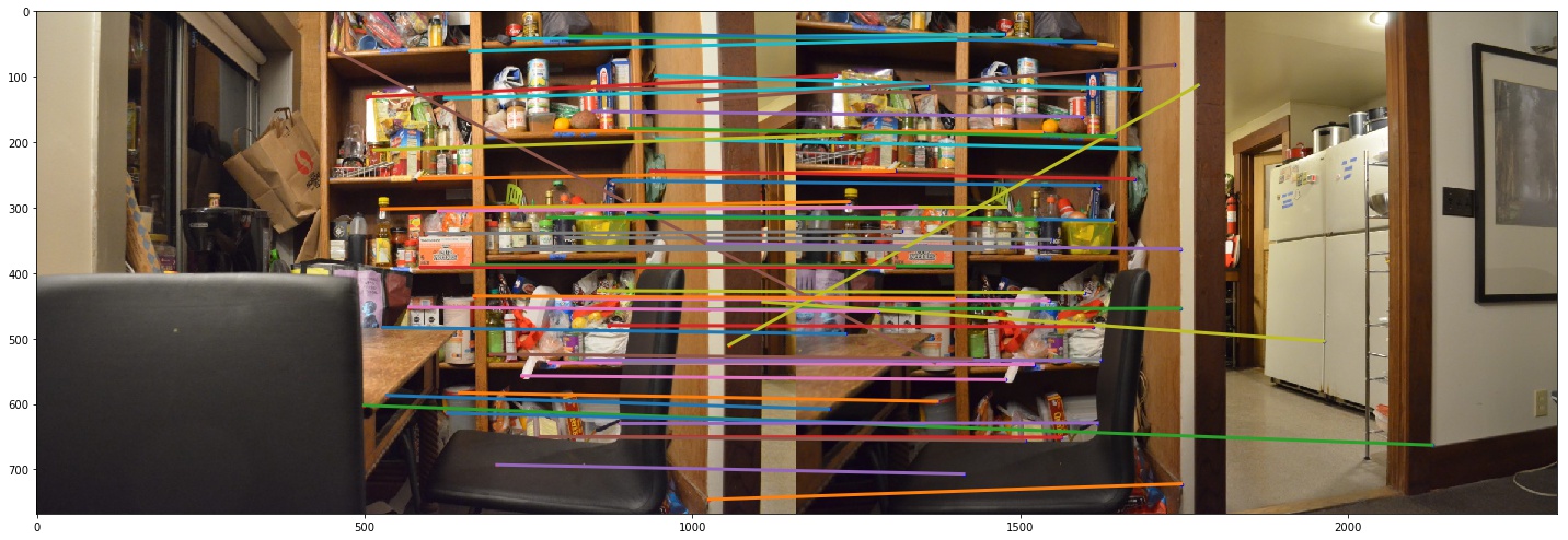
Random Sample Consensus (RANSAC)
The goal of RANSAC is to help us identify the actual, valid feature pairs that will give us the best possible homography. We do this by repeating the RANSAC algorithm many times over - in this case, we use 1000 iterations.
In each iteration, we will randomly choose 4 pairs of correspondence points from the previous step, use these 4 pairs to compute a homography, apply the resulting homography to all of the interest points in the first image, and finally check how many of those points were transformed accurately. Accuracy is measured by how close the transformed points of the first image are to the location of their corresponding points in the second image (i.e. using the L2-distance).
Over many iterations, we will track which was the largest subset of points that was accurately transformed. We will then keep these points to compute the final homography. Intuitively, this works because we assume that no single homography will satisfy all the incorrectly matched pairs (i.e. we assume they're all mismatched in different ways), but correctly matched points should all transform accurately with the same homography.
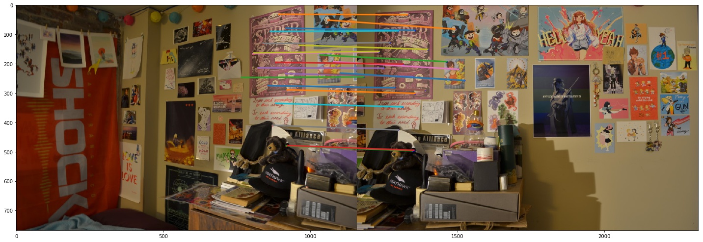
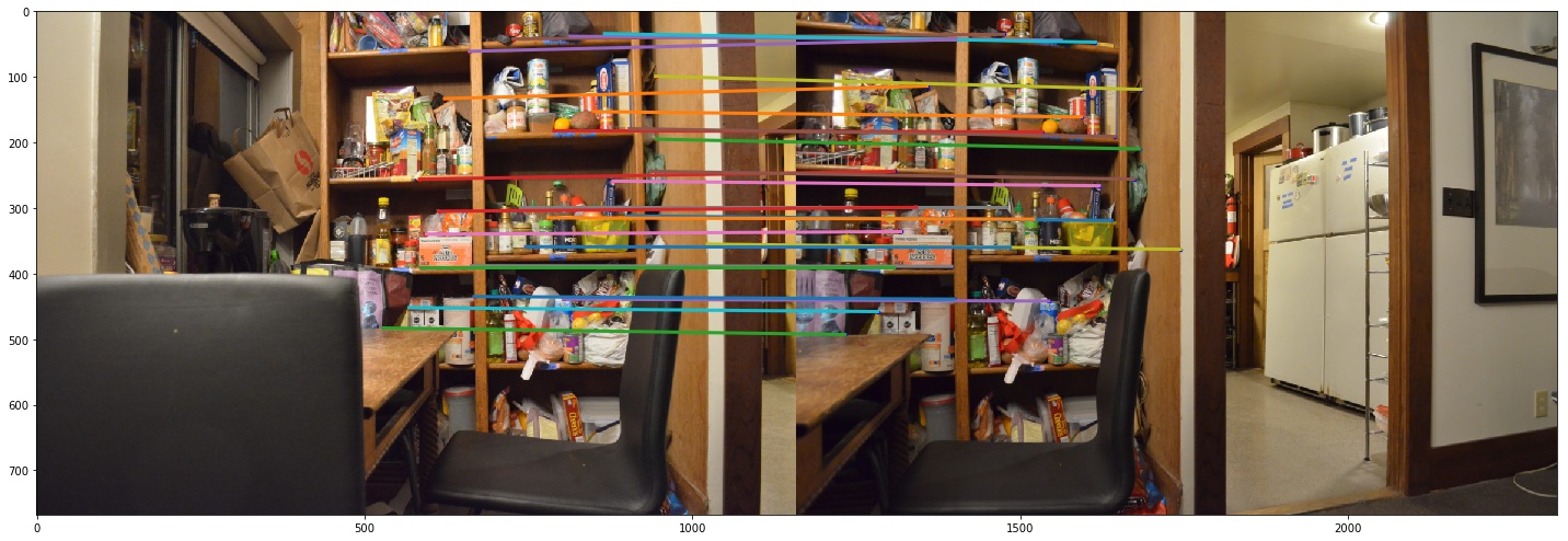
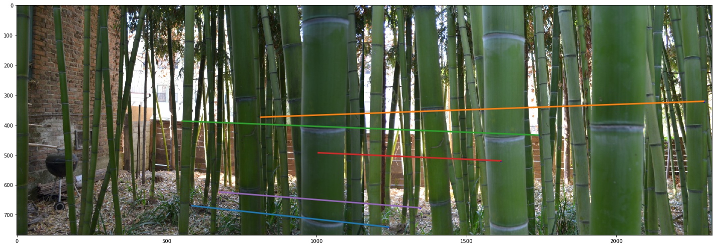
The following images show the final correspondence point pairs.
Final Results and Reflections
Let us compare the panoramas generated using the final correspondence pairs found via RANSAC against the panoramas generated using manually selected correspondence pairs.
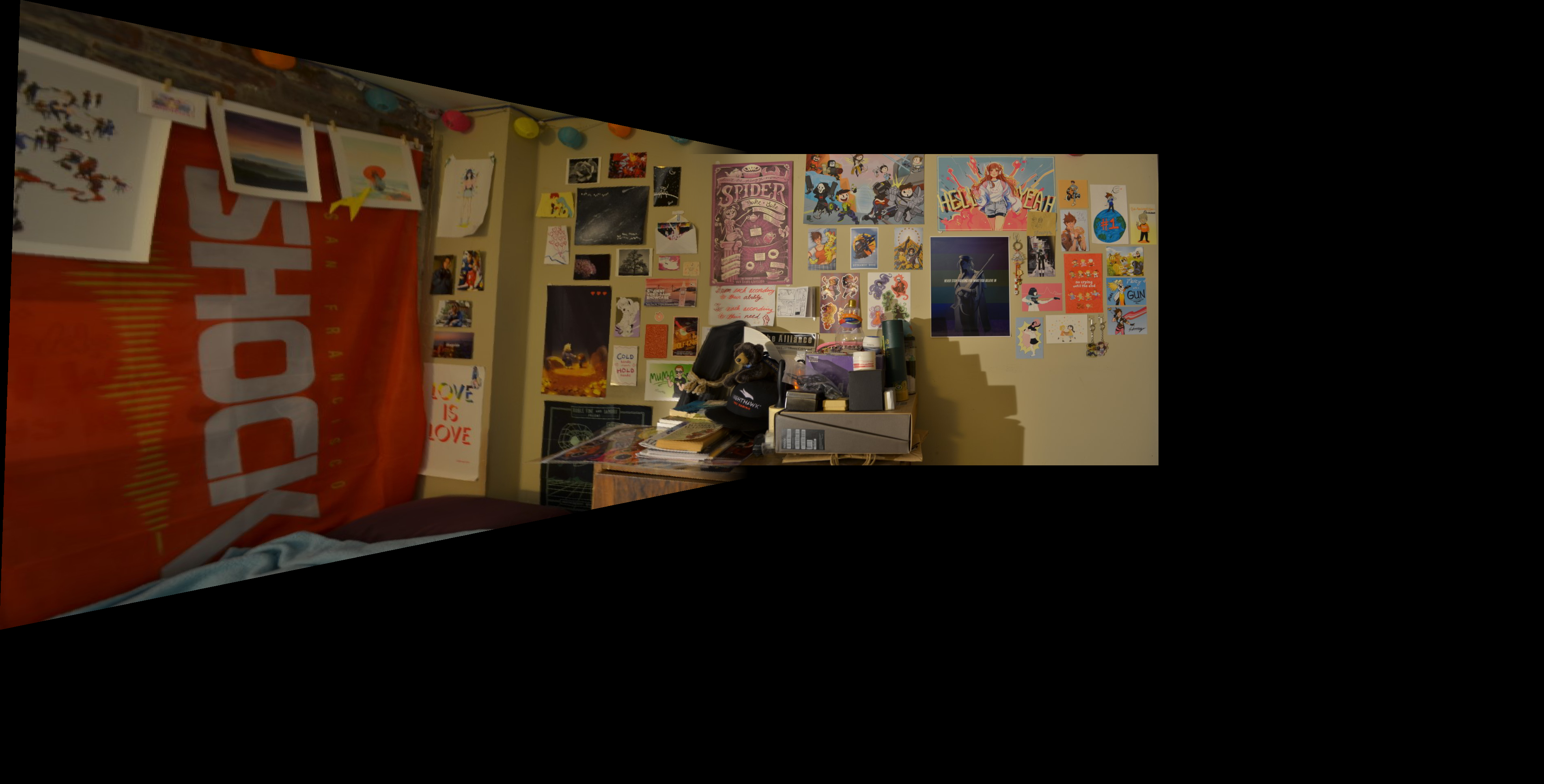
In this panorama, we can see that the auto-generated points produced a much less "slanted" warp for the first image than the manually selected points. We can also see that the purple "Spider" poster near the middle of the two images is much better aligned using the auto-generated points than the manually selected points. If one zooms in, you can see that the manual panorama has some blurriness/ghosting on the poster from misalignment but the auto panorama has much, much less. Clearly this is one benefit we can get from auto-selection of points: our points can be selected much more precisely, without this room for human error!
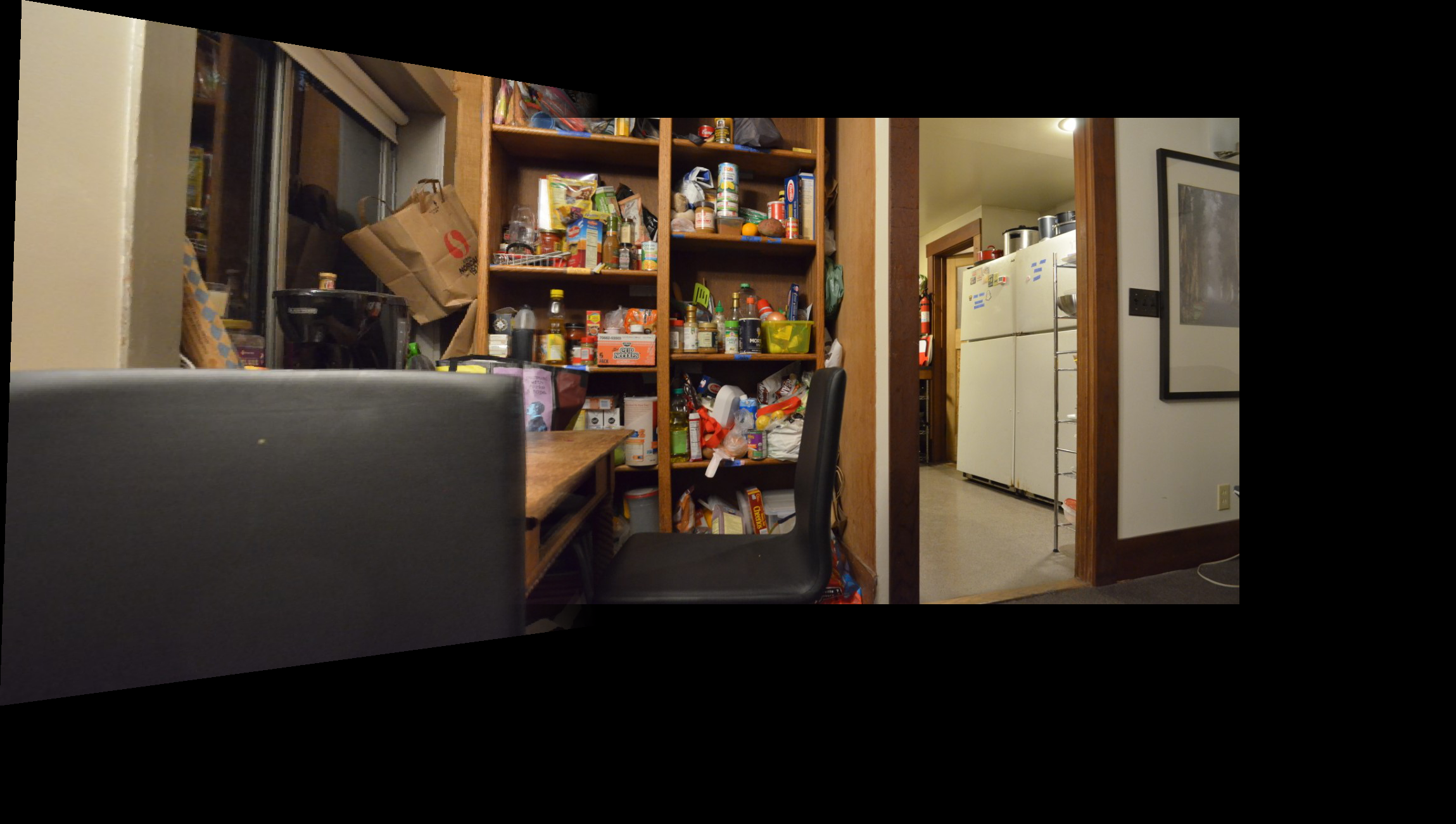
In this panorama, there is not a significant difference in performance upon first glance. One could argue the edge of the black chair on the left near the center of the two images is a little less blurry in the auto panorama than in the manual panorama, but it's difficult to perceive regardless.
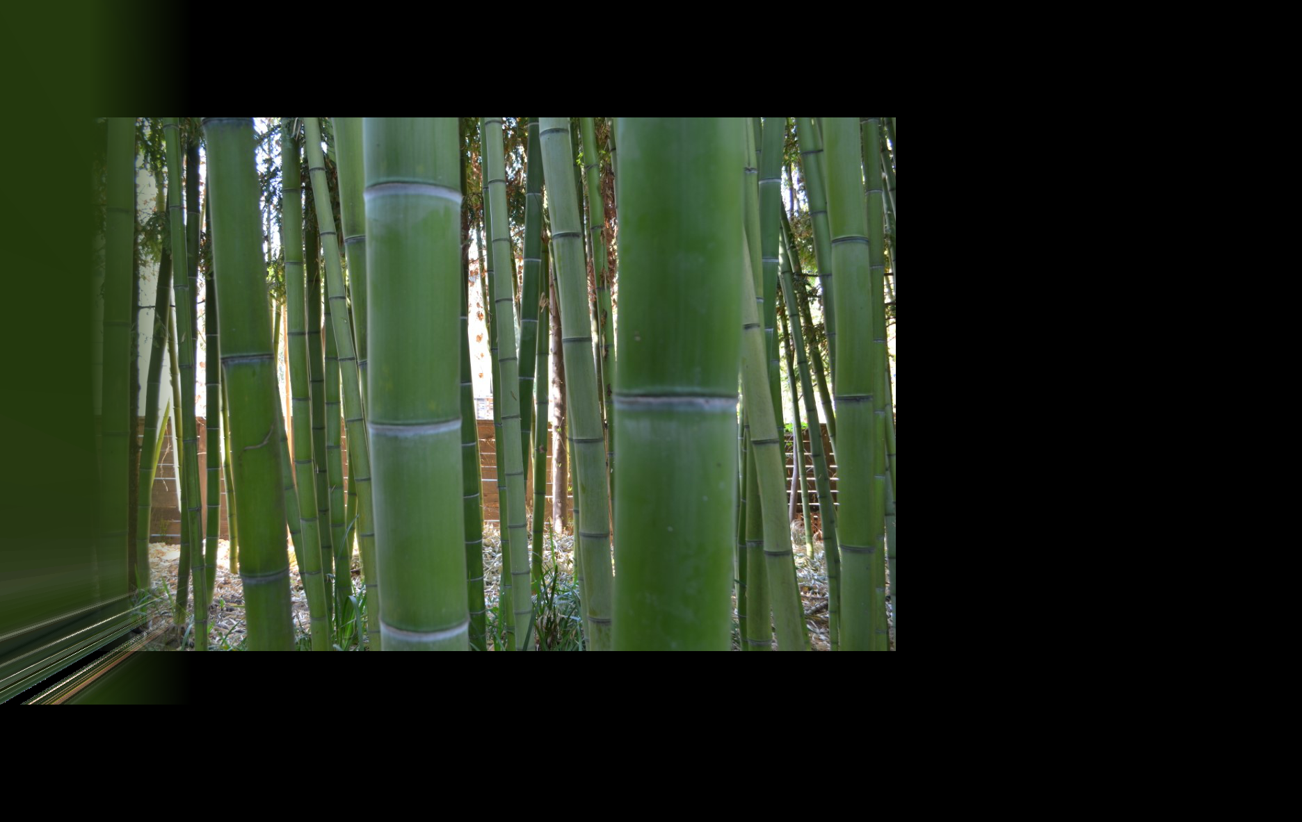
Now this was a result that surprised me. After seeing two previous auto panoramas turn out remarkably well - in fact, "Room" panorama turned out much better than the manual panorama - it was surprising to see this bad of a failure case. The first image barely even exists and is almost a complete blur in this panorama! But if we go back to the Feature Matching and RANSAC sections, this result isn't that shocking.
Firstly, it's clear that Feature Matching gave the Bamboo scene noticeably fewer matches than for the Room and Pantry scenes. This meant that, whatever points get pruned after RANSAC, we'll be left with relatively few correspondence pairs - only 5, in fact! In the manual matching, there were at least 8 pairs! As a result, the homography that results from the auto-selected pairs will have had less data available to overcome the noisiness inherent to pairing these features at all.
Secondly, if we look at the RANSAC results again, we see that there are still a lot of inaccurate pairs, where the features matched are not features of the same object(s) in the scene. Why might this be? It is quite likely because this scene features a lot of repetitive features (that is, all of the bamboo stalks look really similar). Thus, Feature Matching doesn't get enough information to distinguish between two distinct stalks when we're only using a downsampled 8x8 patch around a point. This might be why we had so many fewer pairs from Feature Matching, because not enough points' patches were distinct enough to separate one neighbor from the next. RANSAC cannot solve this issue alone in this case, because it's simply looking for the best homography under the assumption that the best pairs actually map to the same object and the worst pairs uniquely mismatch objects together. But in this case, there are so many bad pairs from Feature Matching that RANSAC cannot be particularly effective.
What's the coolest thing I learned from this project?
There were many interesting heuristics discussed in the "Multi-Image Matching using Multi-Scale Oriented Patches" paper that we used to create this automatic correspondence-point detection. The most interesting was probably the RANSAC algorithm because of the way it very effectively prunes the correspondence pairs just by sampling a few points at a time and testing out the samples' homography. We manage to go from a somewhat noisy set of correspondence points to a simplified, fairly robust set in a relatively short amount of time, even when we iterate up to 1000 times. It's fast and works well, and that's really cool.
What's more, I think, is realizing through analyzing my own failure case is that, even if they come from an Official Research Paper™, these algorithms still have plenty of room for improvement. And it's cool that there are still plenty of avenues for future research into better heuristics for extracting descriptors, matching features, pruning matches, etc!
Acknowledgements
Credit to Rohan Narayan for helping me with aligning images for blending.
Credit to Tianrui Guo for spotting an issue with inconsistent data types for my numpy arrays.
Credit to Ajay Ramesh for his helpful visual debugging code available here: https://piazza.com/class/jkiu4xl78hd5ic?cid=348.