|
|
|
|
|
|
This project was using projective transforms to "rectify" images and create mosaics and panaromas. The steps were: shoot pictures, recover homographies, warp images, and blend images into mosaics.
Here are some pictures of linear interpolation with various C values
|
|
|
|
|
|
|
|
|
This is the matrix H such that for each point p1 in image1 to its corresponding point p2 in image2, you can get the relationship p2 = H*p1. This is a 3x3 matrix that does the perspective transform on each point of the original point. To construct this H, I used eight corresponding keypoints between each picture for mosaics and four corresponding keypoints for rectifying images, since you just need a rectangle.
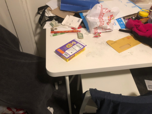
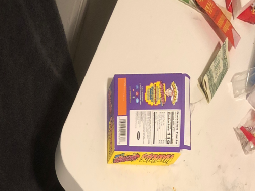
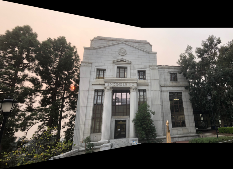
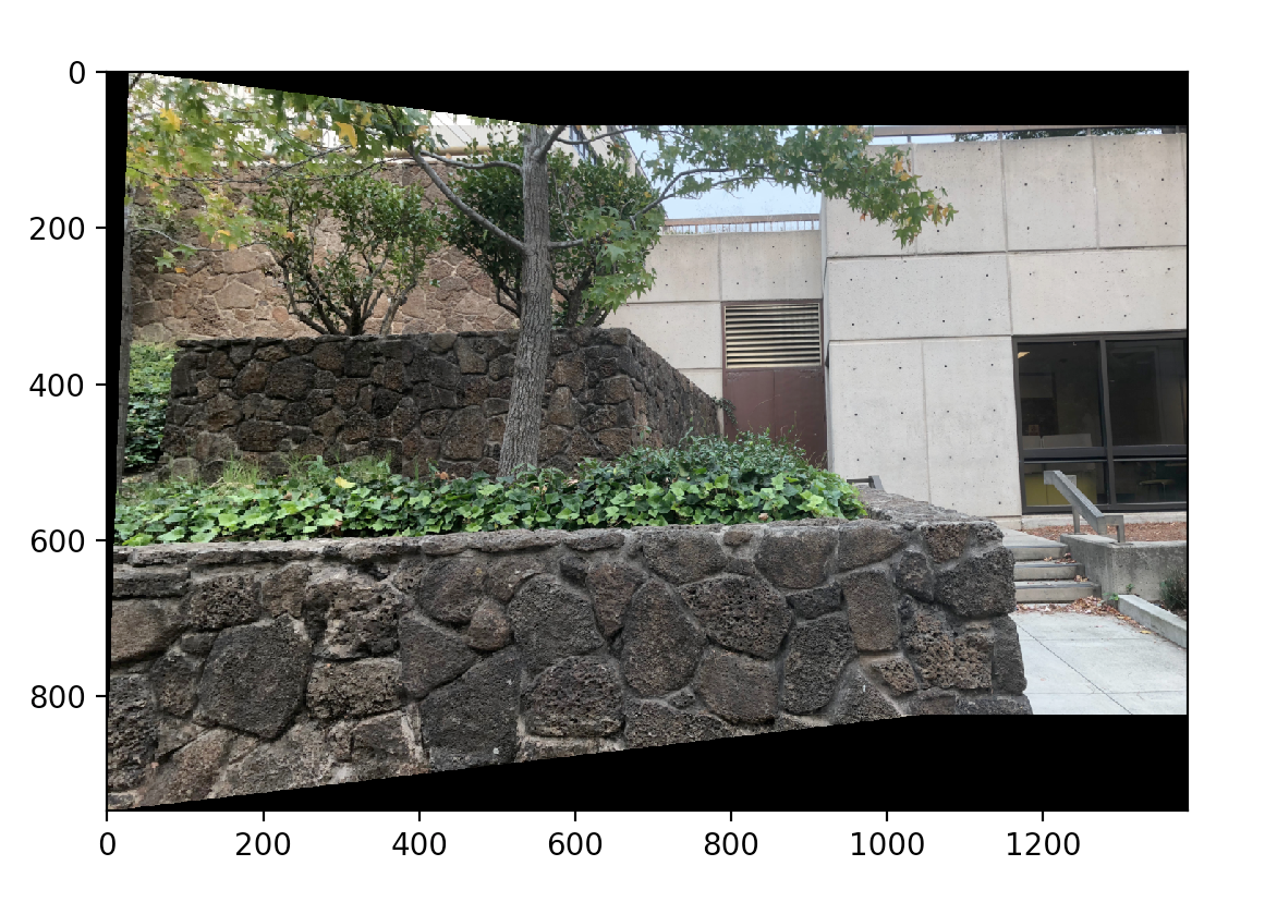
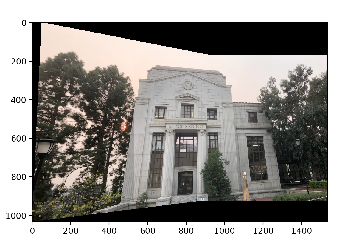
Continuing on about what I stated above, "rectifying" images involved finding 4 keypoints of a warped rectangle (let's say a piece of paper that is lying down on a table and the camera is looking at it from the side), matching those keypoints to a rectangle (let's say now you're looking at the paper from bird's eye), and warping. Here are some cool images!
Here are some pictures of linear interpolation with various C values
|
|
|
|
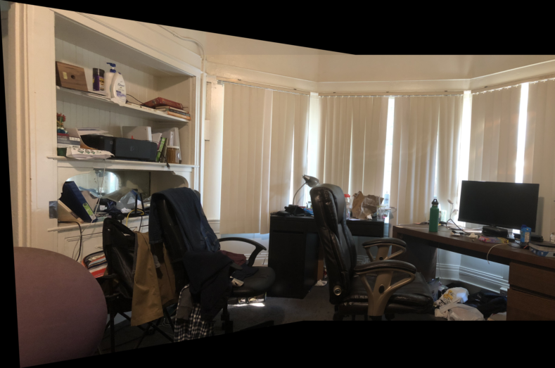
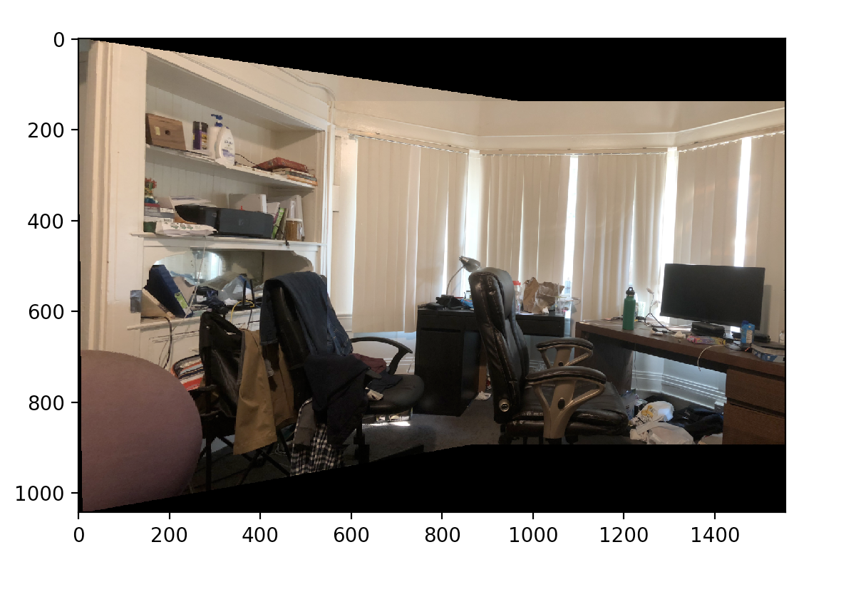
This is essentially what the previous steps (finding homography, warping) led up to. Now, we can blend images into a mosaic. One way that you can do this (which is how I did it) is to have two images, warp one image into the other (say im1 is the warped one and im2 is the unwarped one), and use classic blending techniques to create a mosaic from im1 and im2. You can do this through laplacian, average blending, alpha blending, or simple naive blending. I implemented laplacian, but my naive blending, which involves just putting two together in the simplest way possible, looked much better
|
|
|
What I learned is just how iPhones create panaromas; as you turn it 360 degrees, the iPhone takes several instances of the photos with overlap and computes homography and just blends them together. This is pretty amazing.
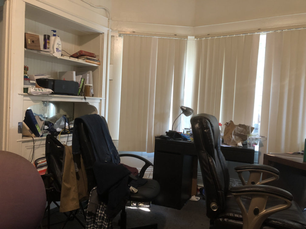
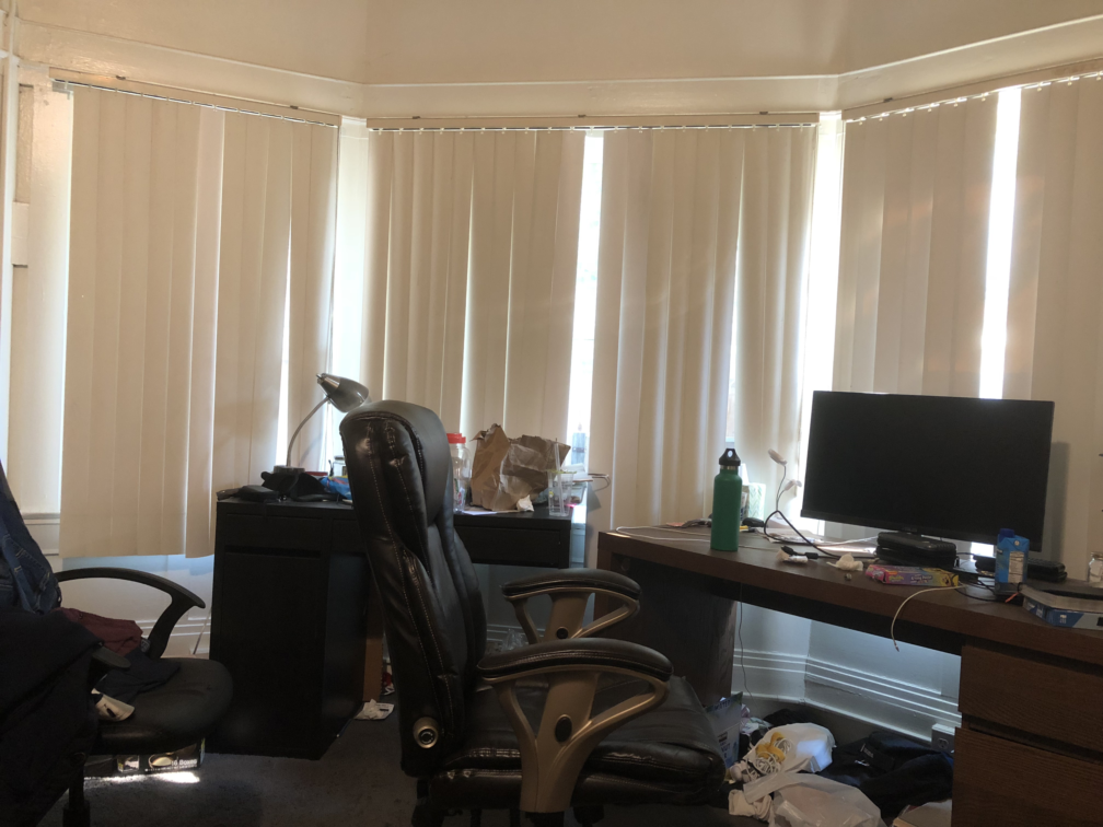
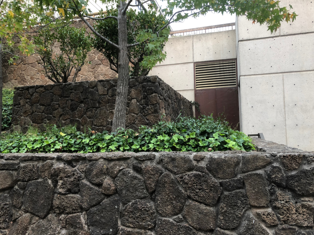
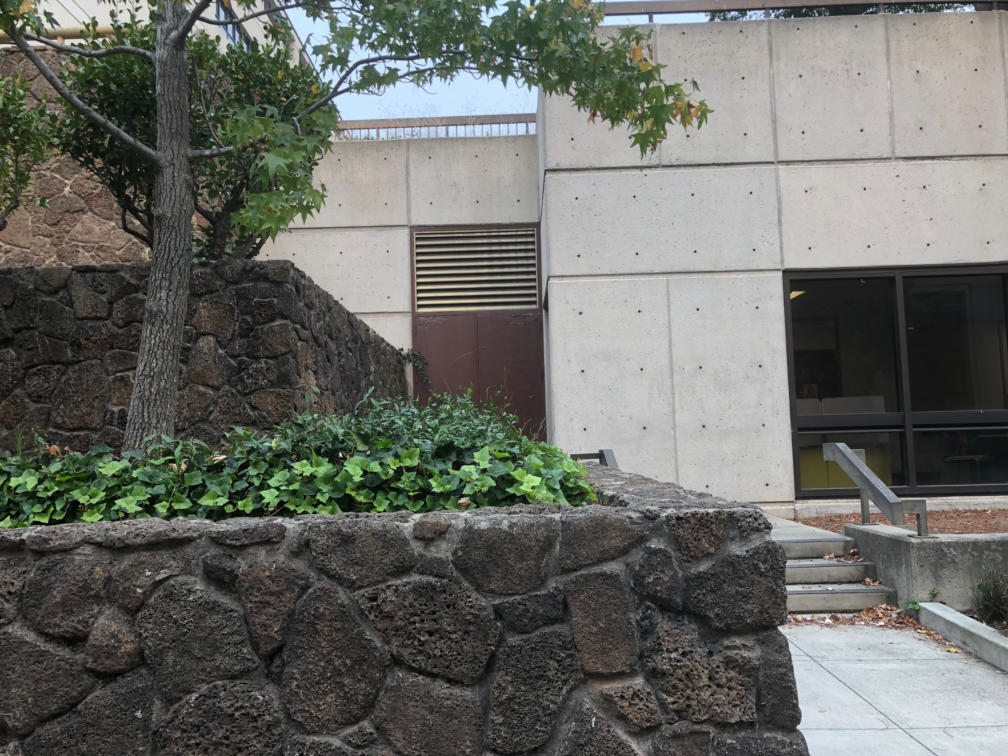
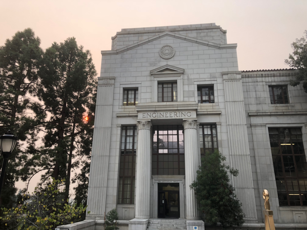
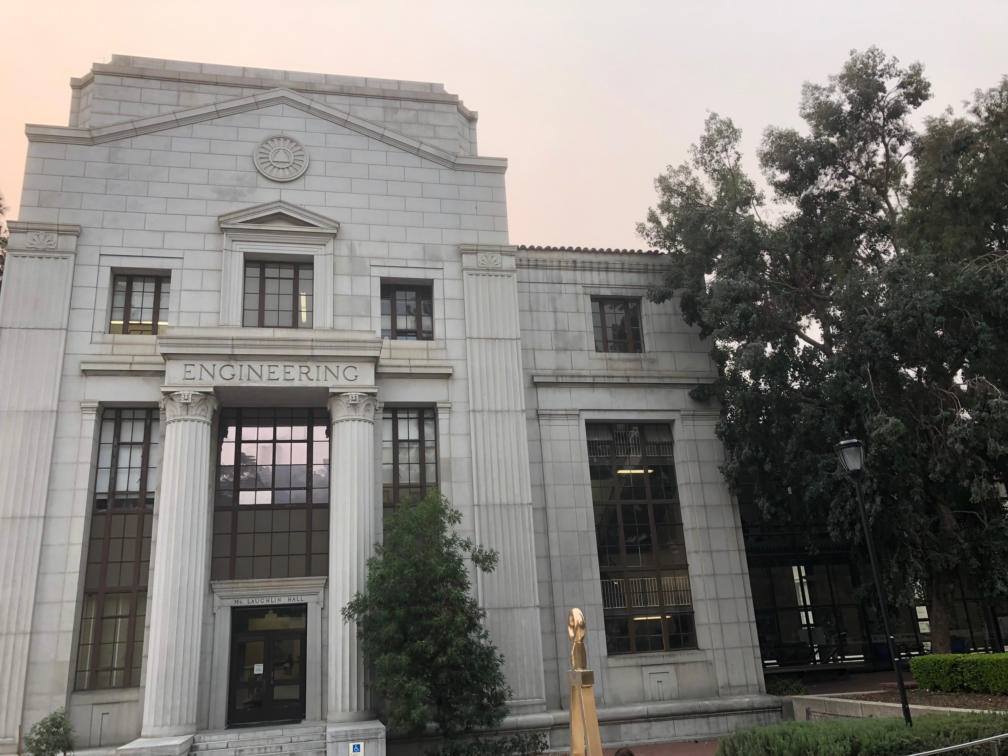
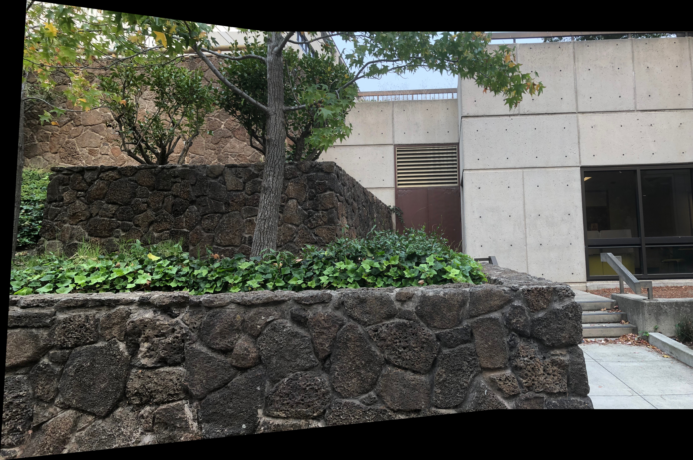
To replace manually selecting keypoints from each picture, since that could lead to errors from pixel rounding and etc, proj6b was to automatically select keypoints that will correspond with each picture. We first start with Harris Corners. For all pictures except the final panarama, I decided to use the "Outside Bechtel" picture.
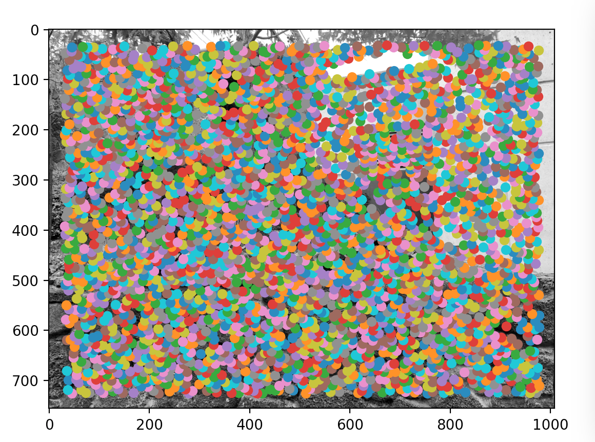
Kinda summarizing †he paper, but for each input image, we form a gaussian pyramid using subsampling rate of s=2 and pyramid smoothing width of 1.0. Then, these interest points are computed from each level. To find these points, we calculate a "corner strength" for each pixel. Intuitively, we can reason this out because we expect corners to be of significance, and to form panaromas, we will be using corners to match picture to picture. Here are some pictures of the Harris corners. There is a LOT of corner points in the beginning (around 3000), and we will use ANMS to pick the 500 most significant ones.
|
|
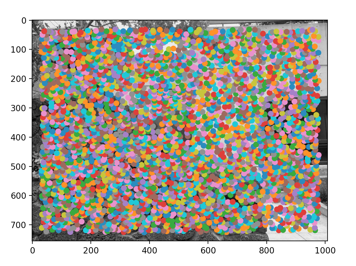
Because there are so many corners (points of interest), we use a strategy called Adaptive Non-Maximal Suppression to restrict the number of interest points. Intuitively, this works by iterating through all the interest points, comparing their "corner strength" with each other, and seeing the "suppresion radius" of each point. Suppression radius is the minimum radius in which a pixel is "overshadowed" by another pixel. If suppression radius is infinity for a pixel, that means it's the global maximum corner strength and vice versa.
Another major intent of this algorithm is to pick strong points that are fairly distant from each other so that the distribution of points will be uniform across the picture. This is important since we don't want all points crowding around one region that doesn't have any overlap with other pictures. Here is my results from ANMSing
|
|
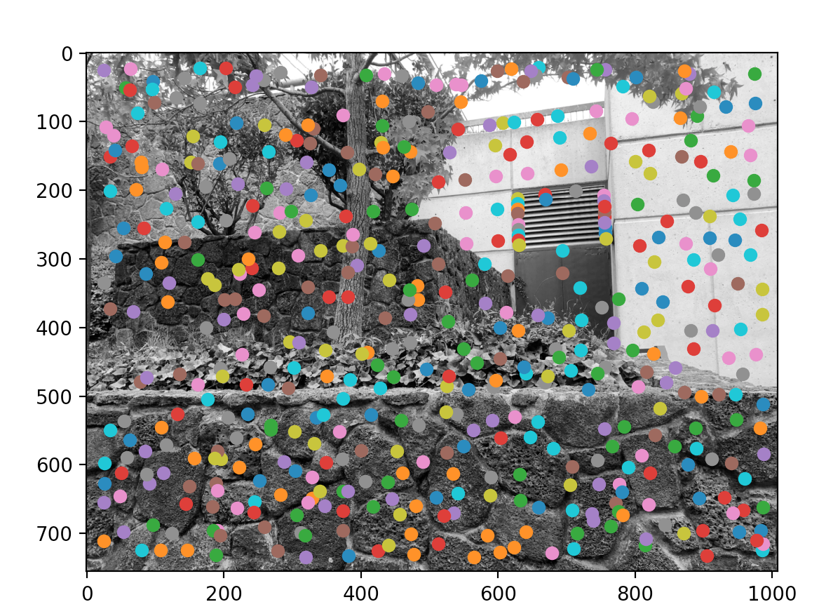
Although we rounded down the total number of possible interest points to 500 per picture, this is clearly too much! To round down more and apply outlier rejection, we first extract features from each point. For the feature, we first obtained the 41x41 window around the point (p[-20+x:21+x, -20+y:21+y]) and prefiltered and downsampled to obtain a 8x8 square. Then, we flattened it and did this for all the 500 interest points per picture.
Then, with the corners and features for each image, we first compared features in picA to features in picB by getting the euclidean distance between each possible pair between them i.e. feature1 of im1 to all of features of im2, feature2 of im1 to all of features of im2, etc. Then, for each corner in image1, we found the "nearest neighbor" and the "second nearest neighbor" by finding the least and second least distance per feature of im1. Then, we got the ratio between the distances (nn1 / nn2) and thresholded to a constant. If the ratio is greater than the constant, it means that the nearest neighbor distance is comparable to the second nearest neighbor distance, and we reject it. Else, we save that pair.
From what I can understand, the reason behind wanting a small ratio for nn1/nn2 is that nn1 is the right keypoint pair while nn2 is almost always wrong. Therefore, if the ratio is large, it signifies that the chance that the nearest neighbor point is the corresponding keypoint is low whileas if the ratio is small, it means that the chance is large since the difference between the first likely mathc and the second likely match is massive. This is because we expect outliers to see every point as "similar" enough (hence nn1/nn2 ~ 1) whileas a real keypoint will match really well with one other point and not so well with its second best point; hence, the low ratio.
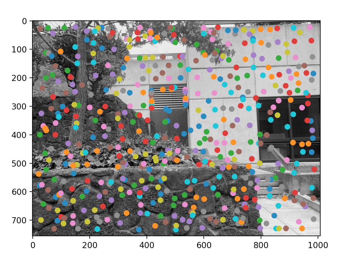
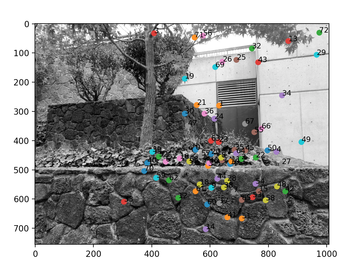
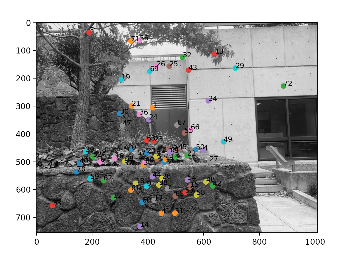
Here are the matching pairs I have found.
|
|
We still have one more process, which is RANSAC. The intuition behind it is that now we have some good keypairs, but there still are some outliers. Now, we will impose geometric constraints by picking four pairs, computing the exact Homography, and seeing how many pairs does the homography work on. We record the number of inliers (the ones that agree with the homography, agree being dist(p2, Hp1) < e for some epsilon error), and we perform this some large number of times. At the end, we take the iteration that produced the most number of inliers, and we perform a least squares estimate of the homography for those inliers.
I used the same pictures for both automatic and manual. Automatic is on the left, and manual is on the right.
Here are the matching pairs I have found.
|
|
|
|
|
|
What I learned is that automatic alignment is so much easier. There are ways to get keypoints from each image, filter out the bad ones, and match the correct ones. Computational Photography has come a long way.