Overview
The main goal of this project is to create panoramas from separate images. The correspondence points are collected one of two ways - manually defined or automatically detected. Once the points are defined in the two images, we use these points to define a homography, which is used to warp one of the images. Once the image is warped, the two images are aligned and blended together.
Collect Images
Task
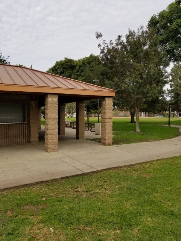
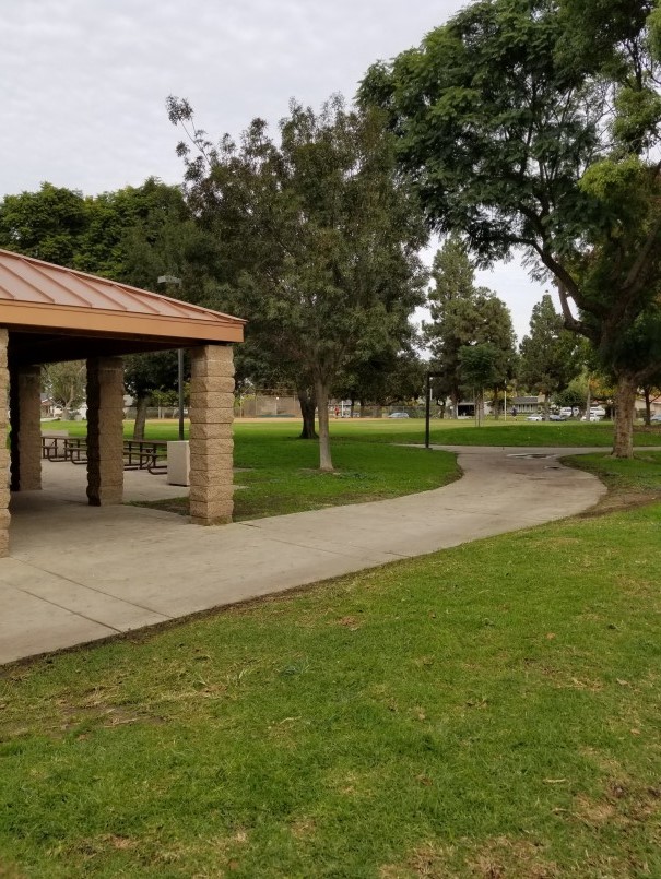
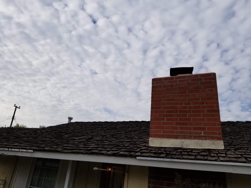
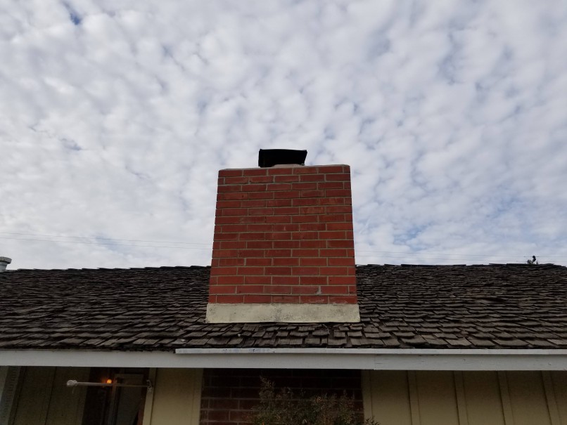
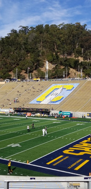
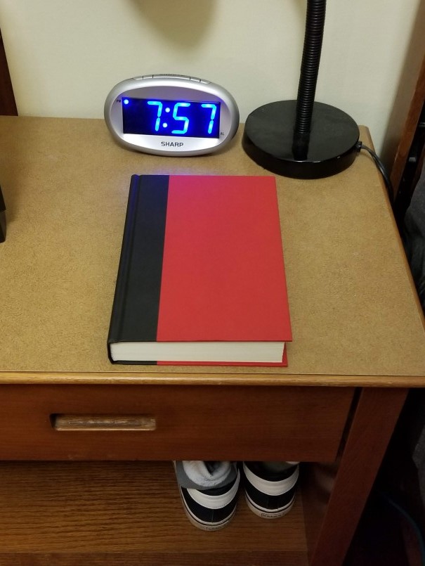
Before we can do anything, we need the images. We need to collect 2 or more images of a particular scene or object from different points of view or perspectives. These images must be collected without translating the camera or changing the settings.
Examples
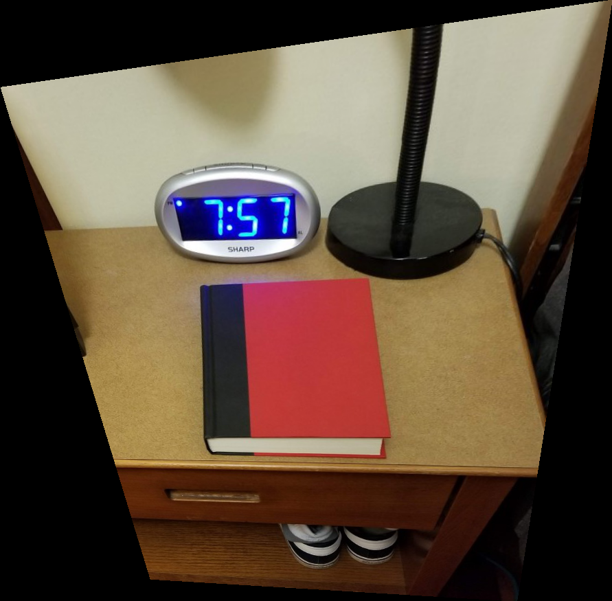
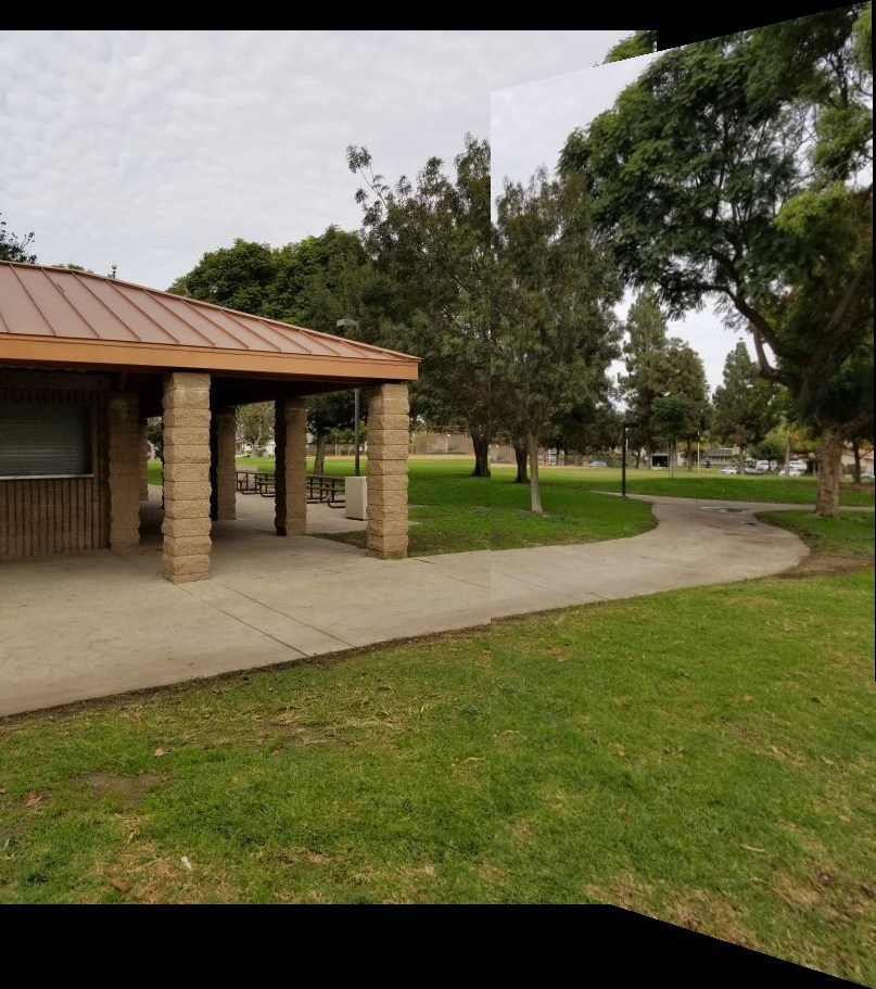
Rossmoor Park
My Roof
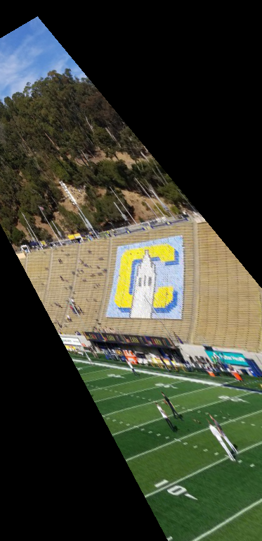
Berkeley
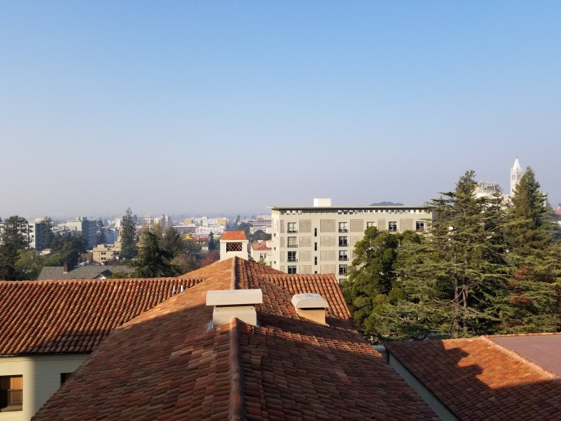
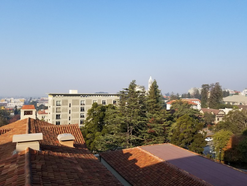
Image Rectification
Task
For this part I manually selected four points on the image and four points defining the goal shape.
I used these points to calculate the homography and I used the homography to warp the original image.
The resulting image shows the defined region warped into the goal shape.
For the following examples I 'rectified' some region of the image.
By warping the image to a certain shape, it changes the persepective so that we appear to be looking straight on to the object.
Results

Automatic Feature Detection
Task
The goal of this section was to automatically detect points for the automatic generation of panoramic images.
The steps followed are based on the paper “Multi-Image Matching using Multi-Scale Oriented Patches” by Brown et al. but with several simplifications.
Harris Interest Point Detector
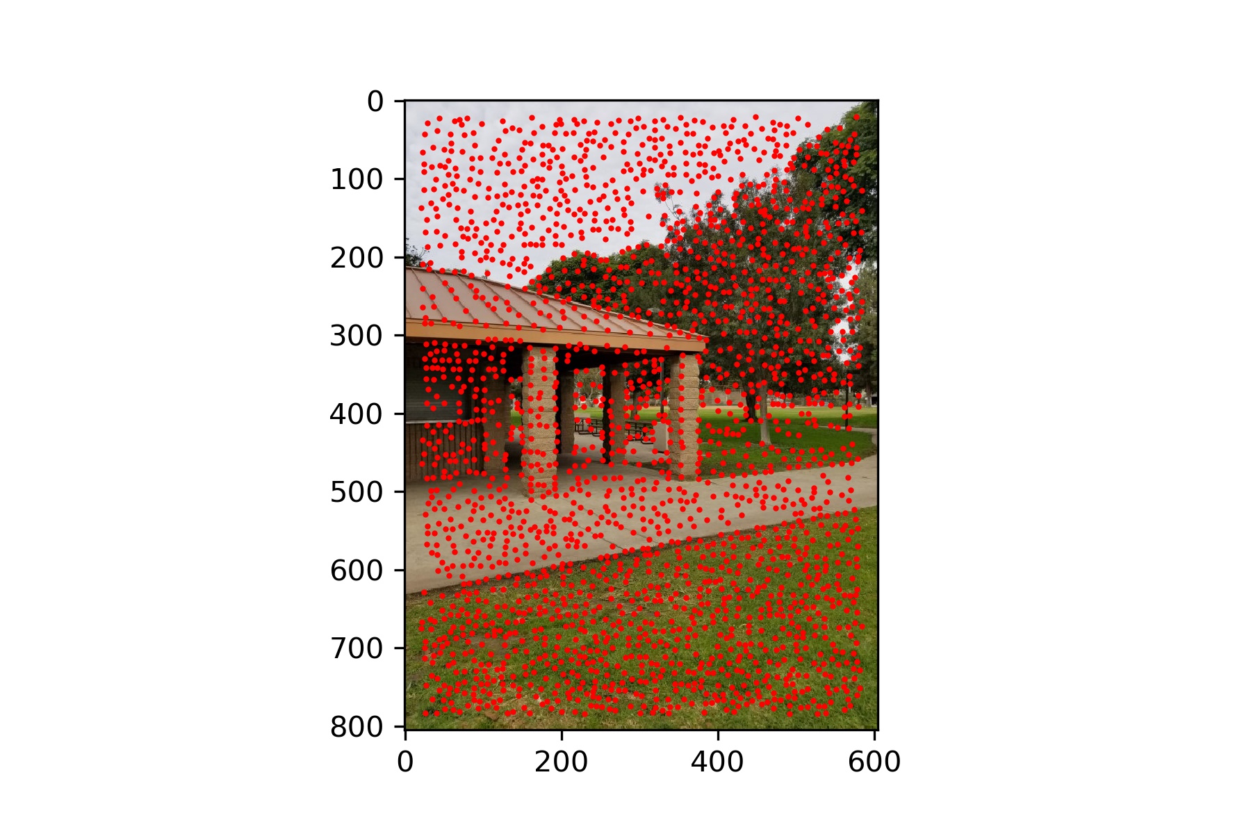
Interest points were generated using the provided function.
The minimum distance was changed to 5.
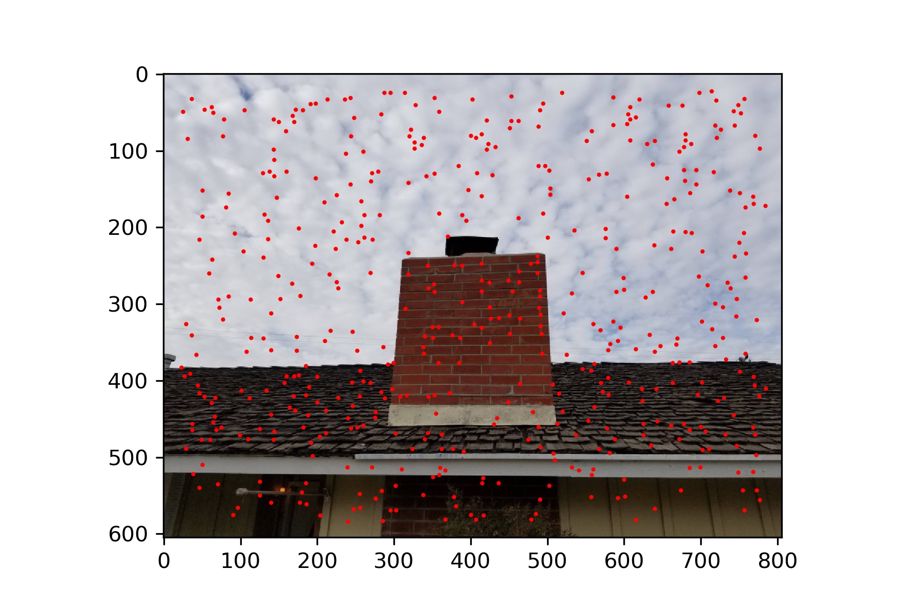
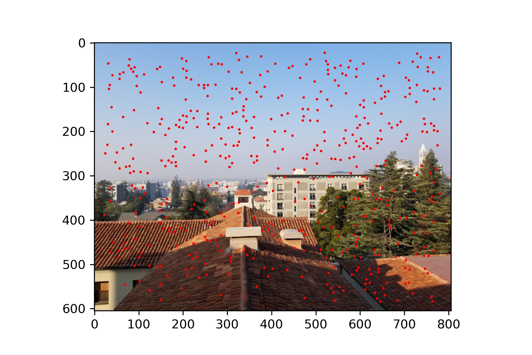
The following images show each of the images with the Harris Interest points plotted on top.
As we can see, we get a lot of feature points after this step.
Rossmoor Park
My Roof
Berkeley
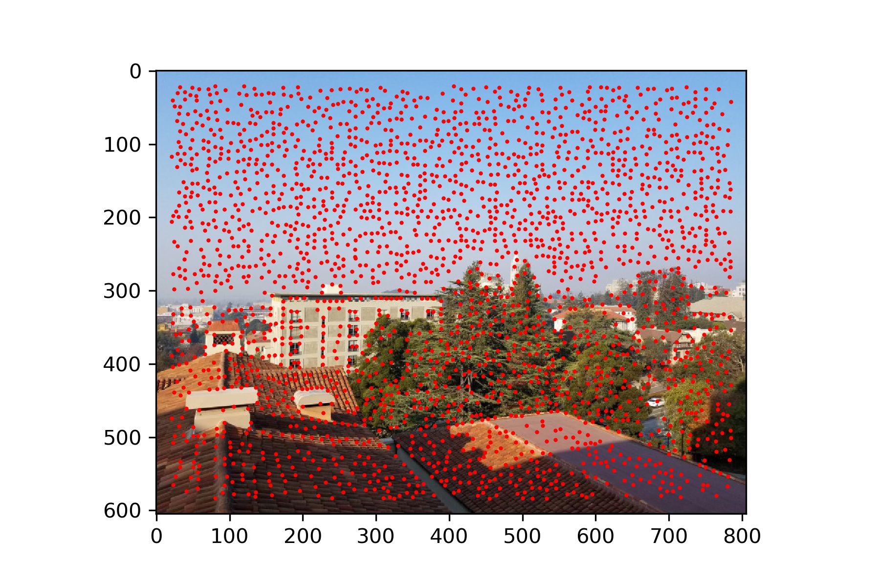
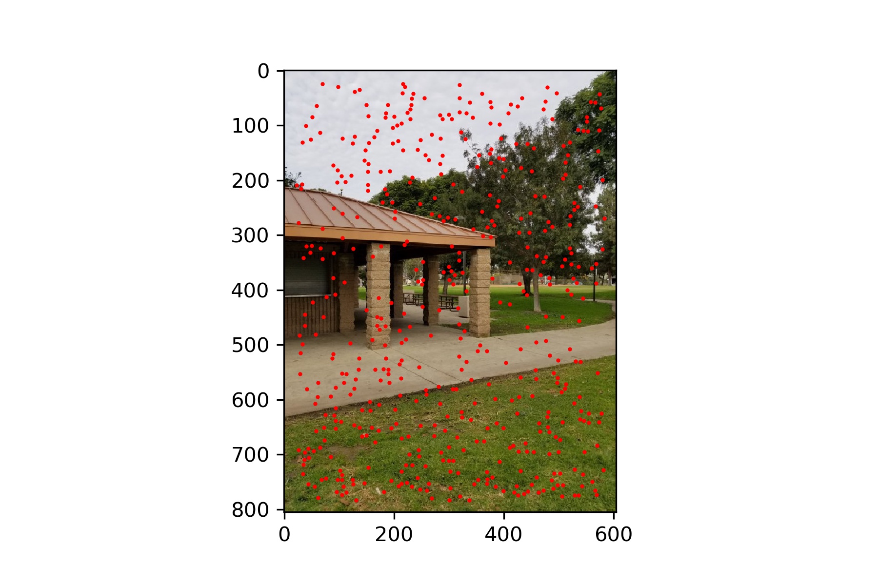
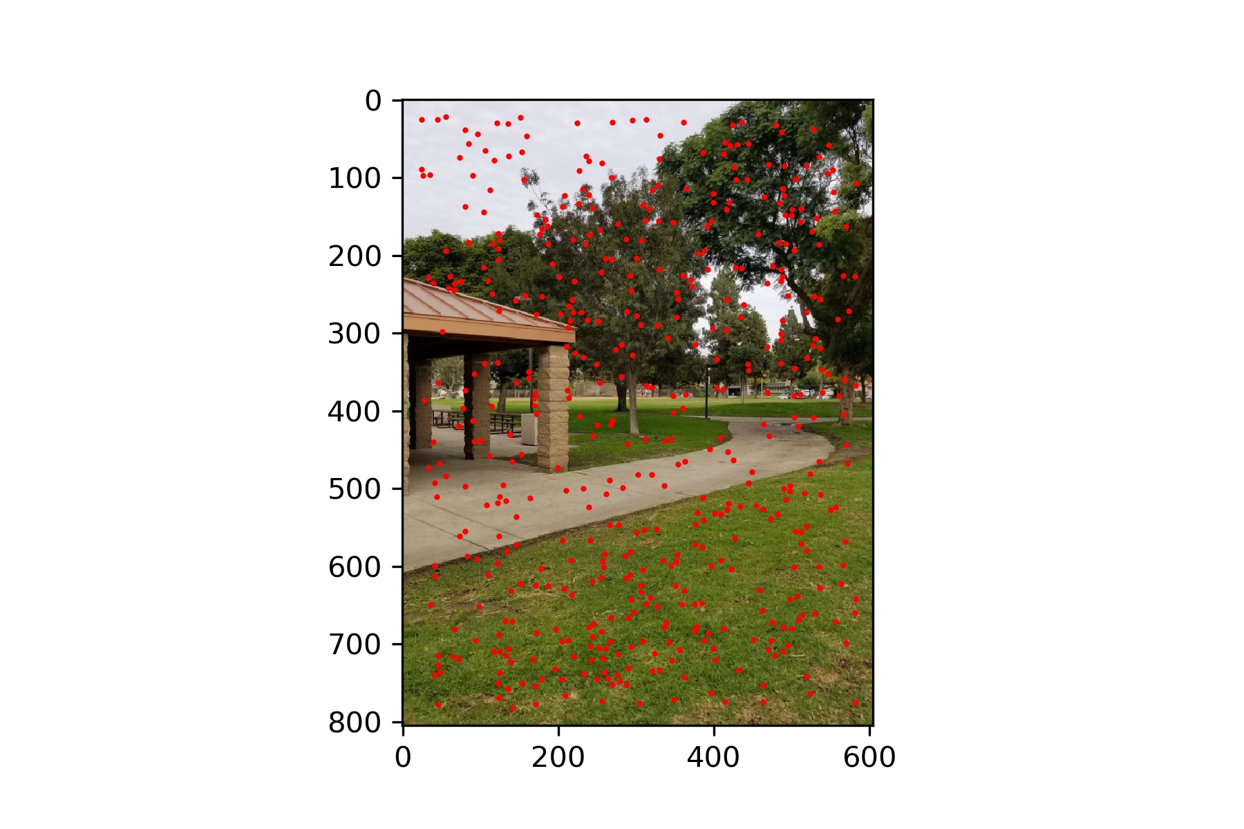
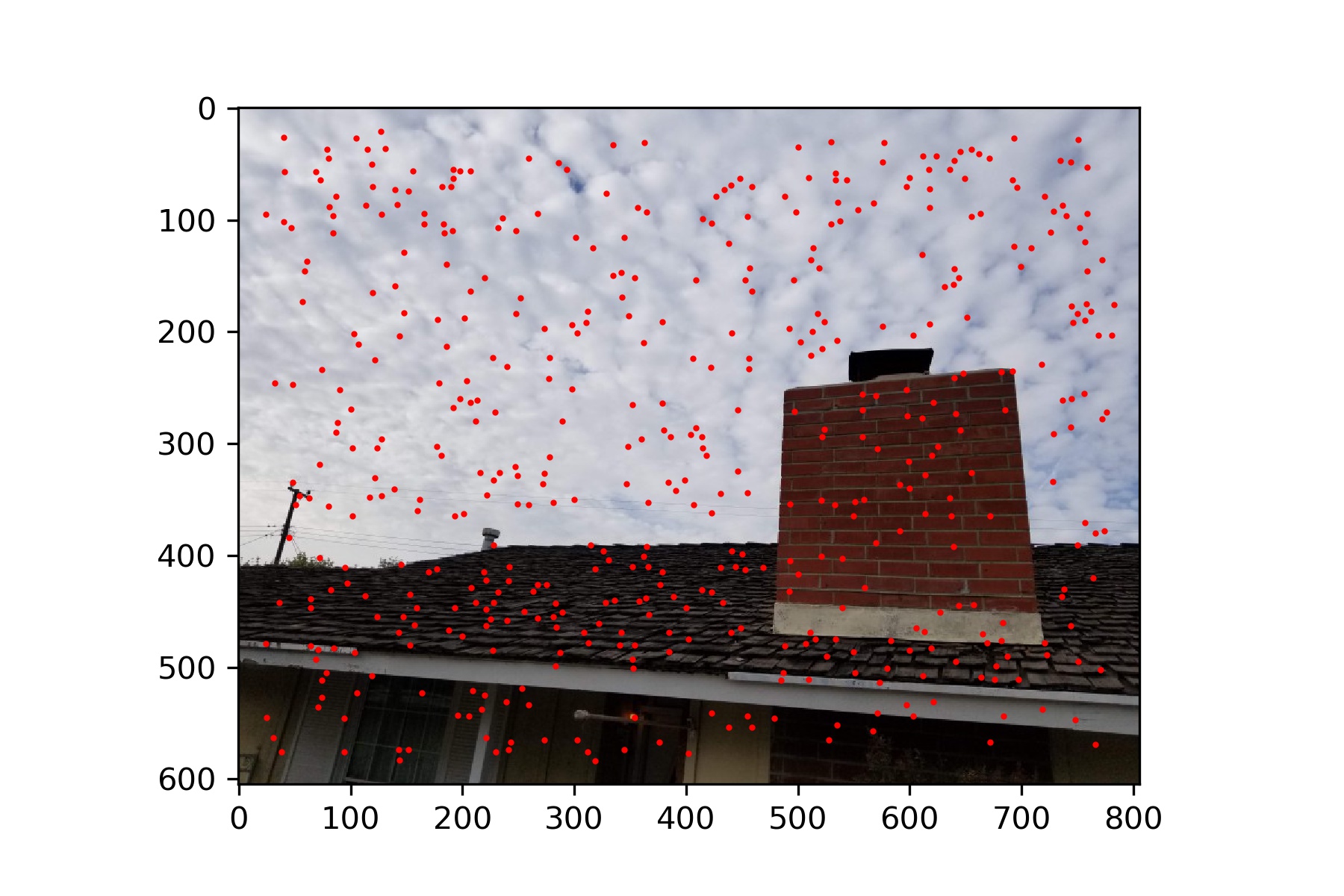
Adaptive Non-Maximal Suppression
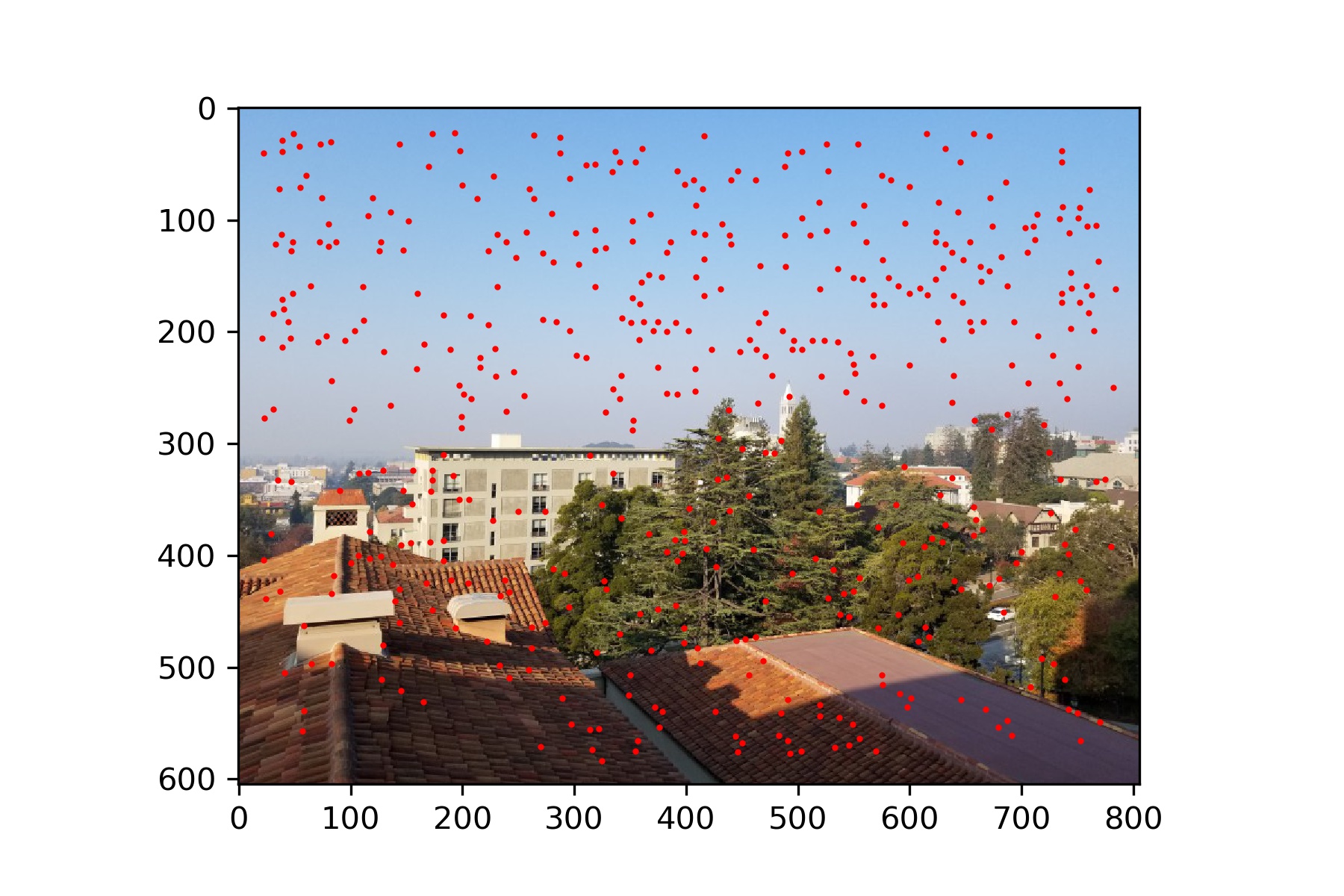
The goal for this part is to narrow down the interest points, so that we have a specified number of strong points that are dispersed throughout the image.
I chose to select 500 points at this step.
It is important that we do not just select the highest strength points, because these points may not be well distributed across the image and thus lead to a loss of information.
The following images show the remaining points after this step. As we can see, there are fewer points than before but the points still spread across the whole image.
Rossmoor Park
My Roof
Berkeley
Feature Matching
After finding the interest points in each image, we need to match points between the two images.
We do this by first describing features for each interest point. Each feature is a 40x40 pixel square from the image, resized to 8x8.
This patch is then normalized so that the average is 0 and the standard deviation is 1.
These features give us a way of comparing similarity between regions in the two images.
We create a set of features for each image, each centered around one of the points defined previously.
Then we calculate the difference between each feature from the first image and each feature from the last image.
We consider two features a match if the ratio of one features nearest neighbor over that same features second nearest neighber is less than some threshold value.
I set my threshold to 0.4. This checks that the feature must be very similar to its first closest match and also very different than its second closest match.
This increases our confidence in the match between the two features.
Below show the two images with the locations plotted of all of their matching features.
Rossmoor Park

My Roof

Berkeley
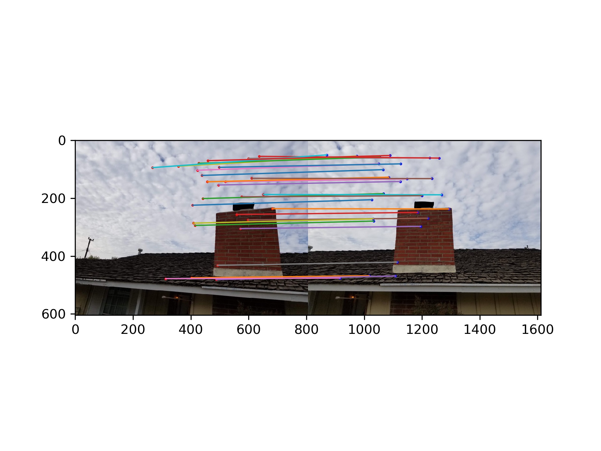
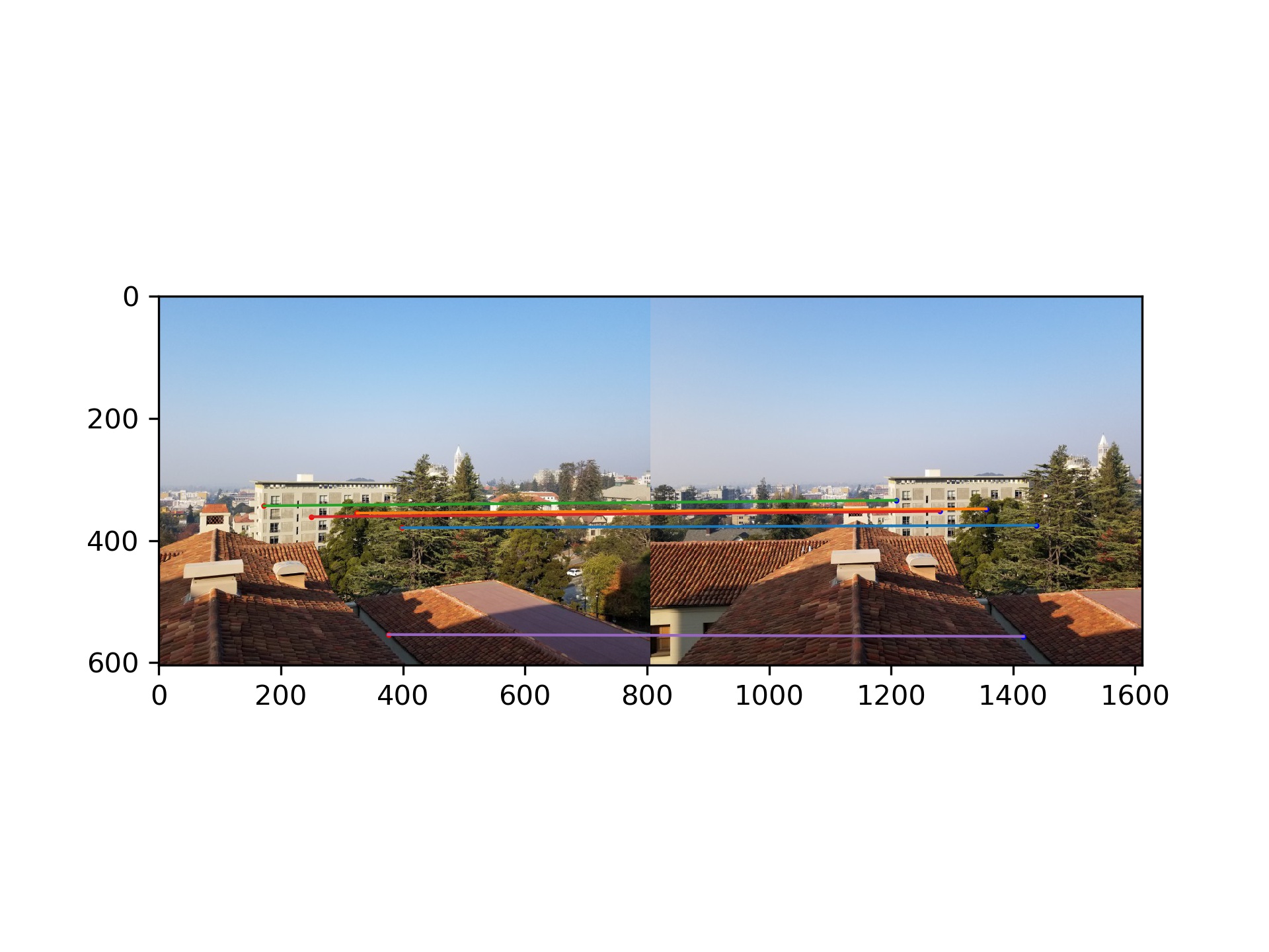
RANSAC
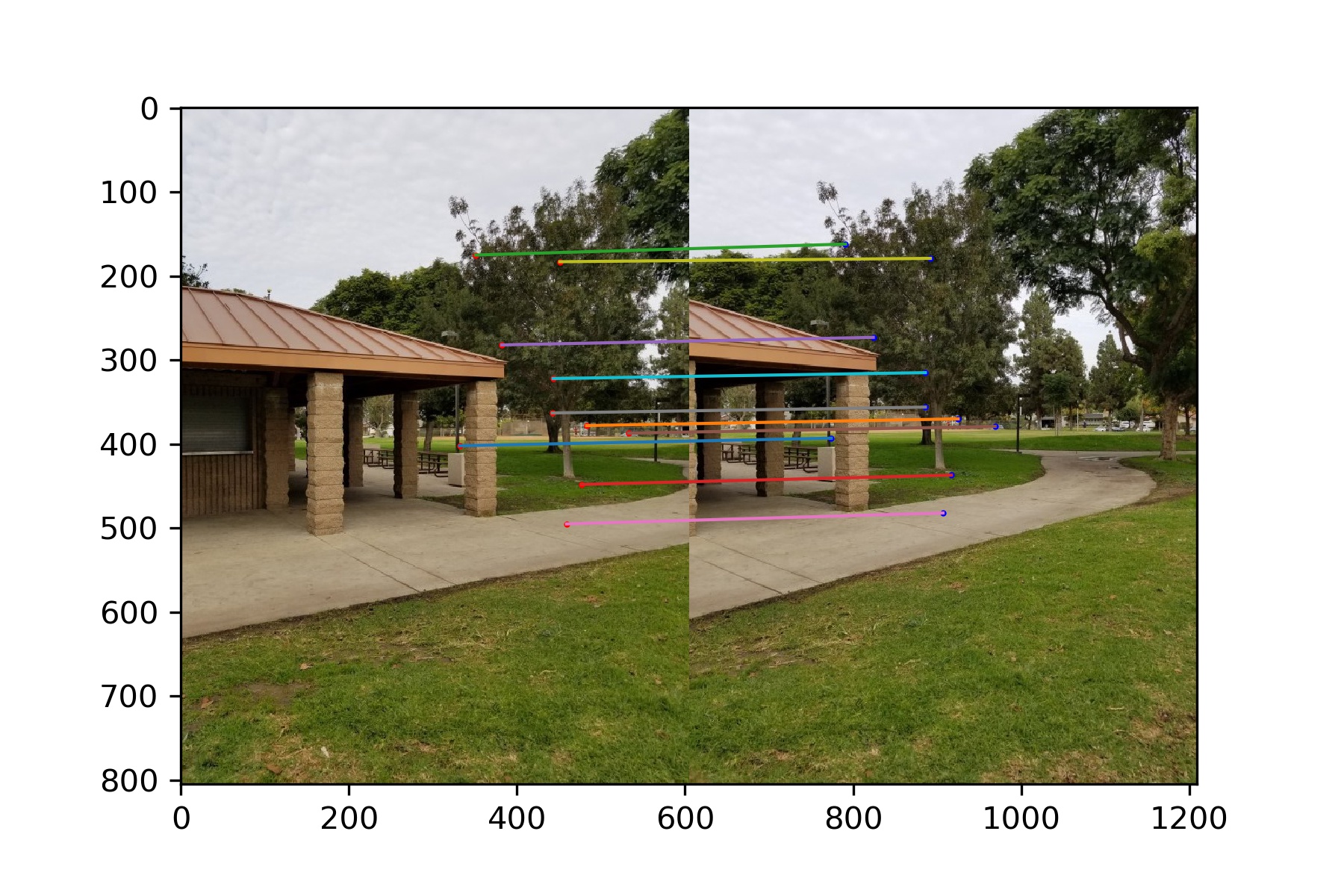
The last step is to further refine our points through the use of RANSAC.
We randomly choose 4 pairs of our matching points and compute the homography.
We then apply this homography to every point from our final set of points for our first image
and calculate the difference between the resulting point and the matching point from the second image.
If this difference is less than some threshold value (I use 5), then we keep this point as an 'inlier'.
We repeat this process many times and retain the largest set of inliers. This helps eliminate bad points.
The theory is that many of the points should be warped to the correct position by the same homography, and those that are significantly off are not well-matched points.
Below are the point correspondences that remain after 200 iterations of RANSAC.
Rossmoor Park
My Roof
Berkeley
Panoramas
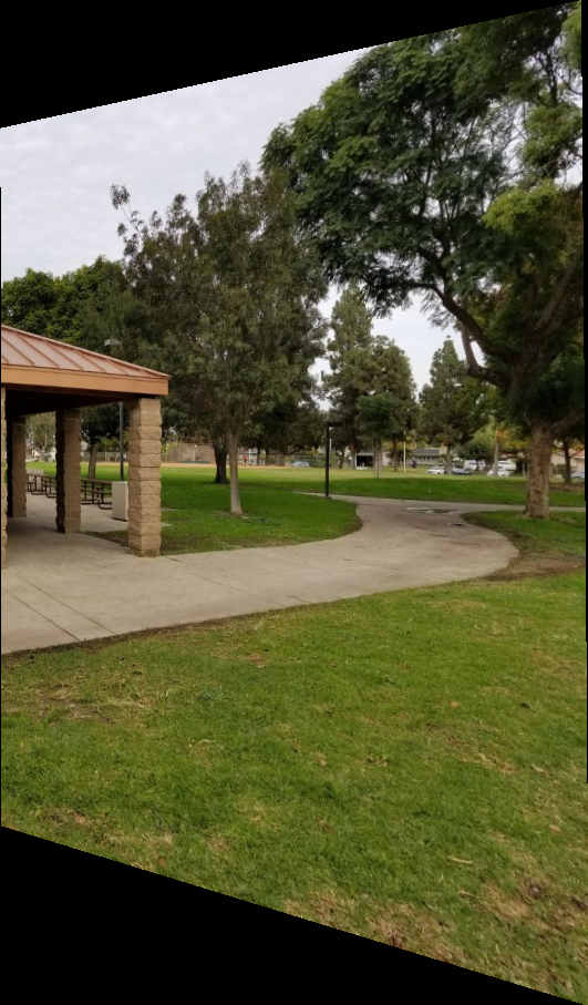
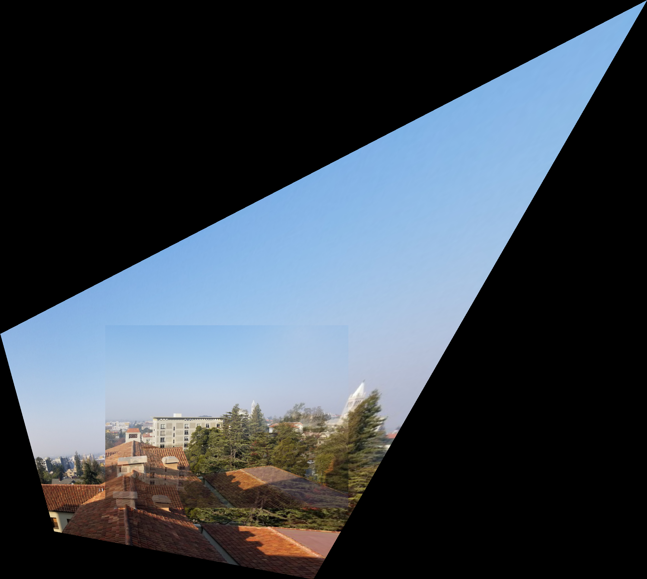
After obtaining a set of point correspondences between the two images, either by manual selection or automatic detection, we use these points to calculate a homography and warp one of the images.
After warping the image, I align it to the other image using the position of one of the points from the first image and the warped corresponding point from the second image.
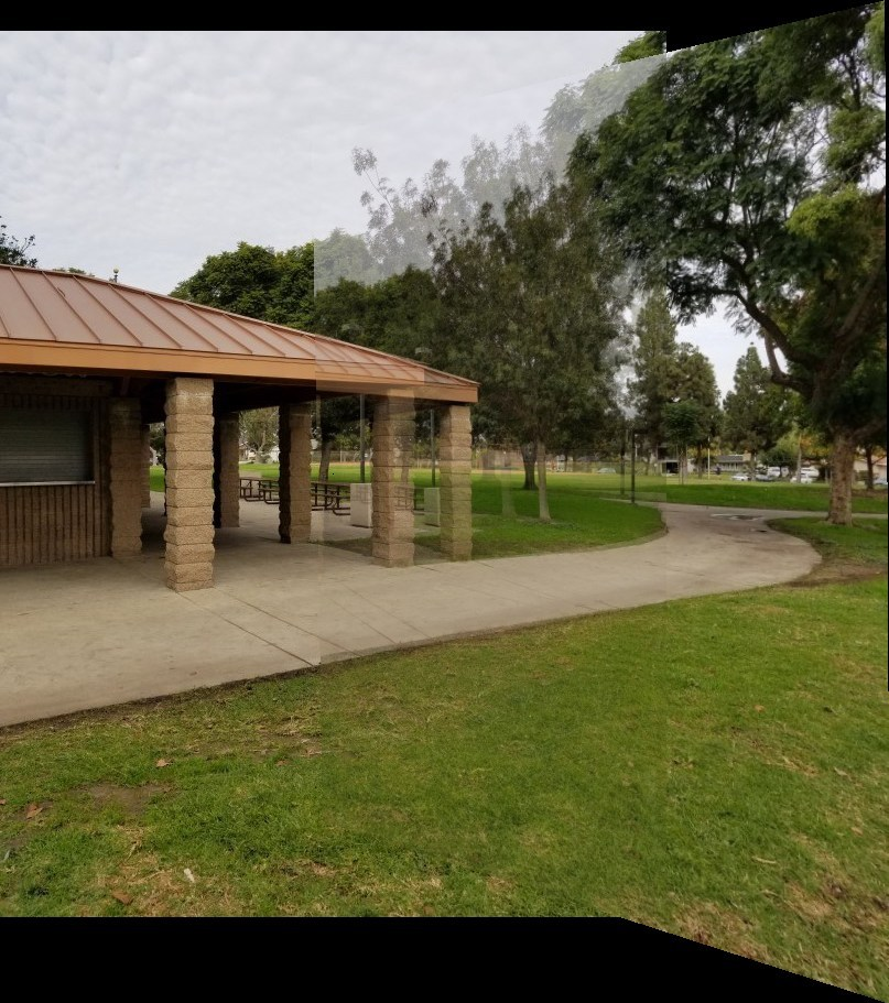
From there I blended the images using a weighted average.
For each pixel I calculated its distance from the center of that image, weighted the value of the pixel from each image by 1/distance, summed the values and divided by the total of the two scalars.
This gives greater weight to those pixels closer to an image's center. As we can see the results do not look good, and this is due mostly to a misalingment.
Additionally, better methods of blending could be explored, such as through the use of Laplacian Pyramids.
Results
Rossmoor Park - Manual points
Warped Image
Panorama
Rossmoor Park - Automatic points
Warped Image
Panorama
Panorama without blending
My Roof - Manual points
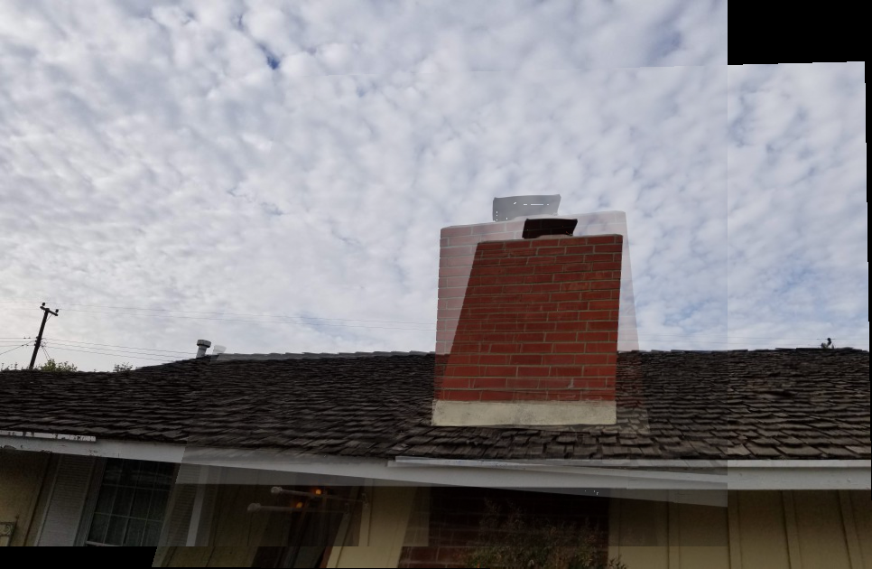
Warped Image
Panorama
My Roof - Automatic points
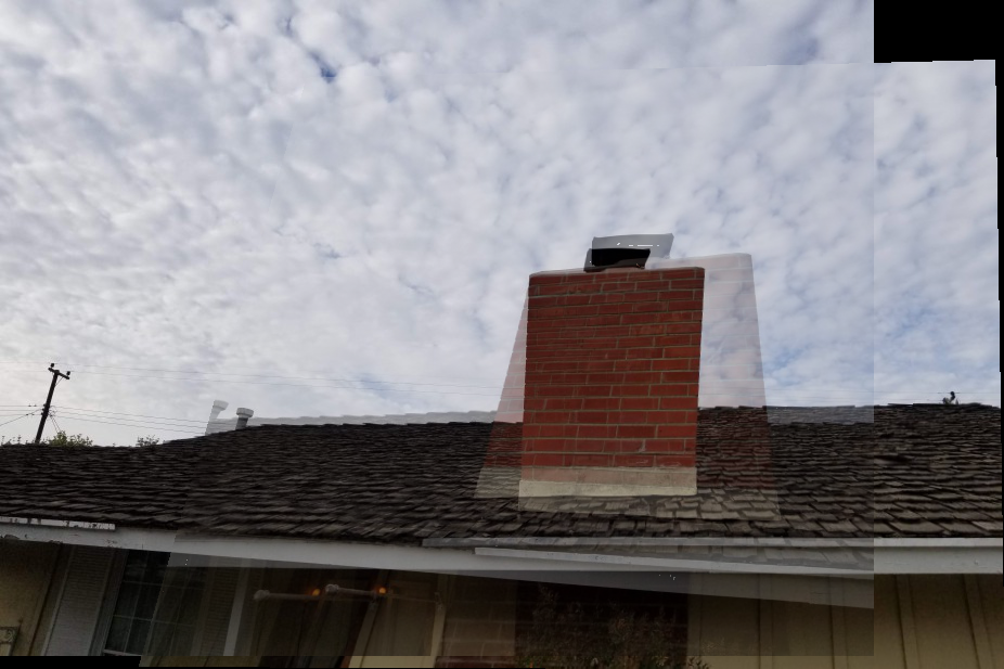
Panorama
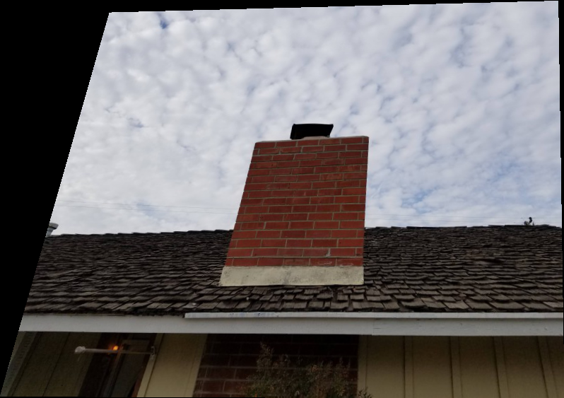
Warped Image
Berkeley - Manual points
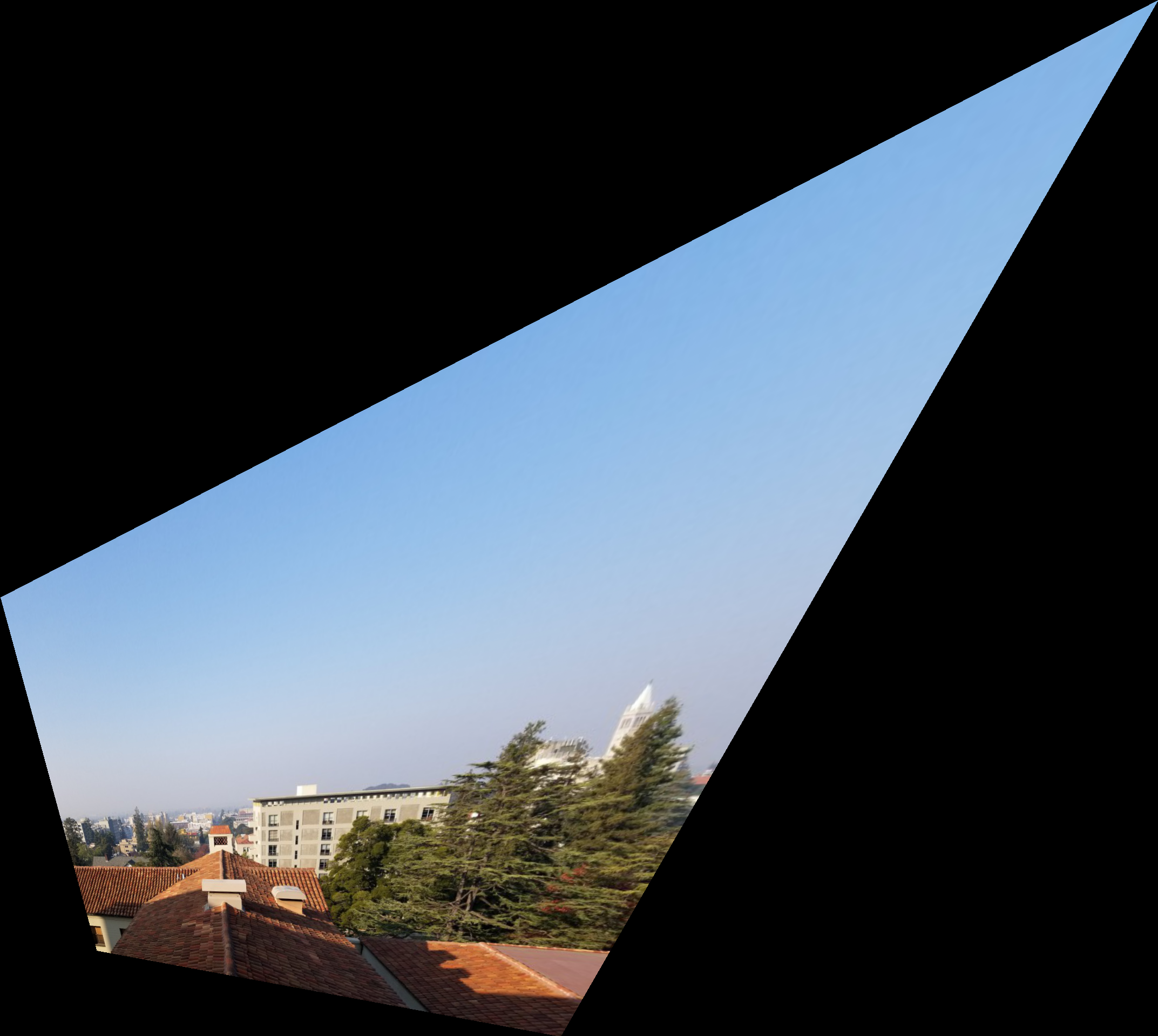
Warped Image
Panorama
Berkeley - Automatic points
Warped Image
Panorama
Conclusion
There is still much work to be done to improve the results, especially with the alignment.
Additionally, the difficulty of this project makes me appreciate the simple panoramic settings on cameras.
|
|
|
|
|
|
|
|
|
Image Rectification
Task
For this part I manually selected four points on the image and four points defining the goal shape. I used these points to calculate the homography and I used the homography to warp the original image. The resulting image shows the defined region warped into the goal shape. For the following examples I 'rectified' some region of the image. By warping the image to a certain shape, it changes the persepective so that we appear to be looking straight on to the object.
Results
Automatic Feature Detection
Task
The goal of this section was to automatically detect points for the automatic generation of panoramic images.
The steps followed are based on the paper “Multi-Image Matching using Multi-Scale Oriented Patches” by Brown et al. but with several simplifications.
Harris Interest Point Detector
Interest points were generated using the provided function.
The minimum distance was changed to 5.
The following images show each of the images with the Harris Interest points plotted on top.
As we can see, we get a lot of feature points after this step.
Rossmoor Park
My Roof
Berkeley
Adaptive Non-Maximal Suppression
The goal for this part is to narrow down the interest points, so that we have a specified number of strong points that are dispersed throughout the image.
I chose to select 500 points at this step.
It is important that we do not just select the highest strength points, because these points may not be well distributed across the image and thus lead to a loss of information.
The following images show the remaining points after this step. As we can see, there are fewer points than before but the points still spread across the whole image.
Rossmoor Park
My Roof
Berkeley
Feature Matching
After finding the interest points in each image, we need to match points between the two images.
We do this by first describing features for each interest point. Each feature is a 40x40 pixel square from the image, resized to 8x8.
This patch is then normalized so that the average is 0 and the standard deviation is 1.
These features give us a way of comparing similarity between regions in the two images.
We create a set of features for each image, each centered around one of the points defined previously.
Then we calculate the difference between each feature from the first image and each feature from the last image.
We consider two features a match if the ratio of one features nearest neighbor over that same features second nearest neighber is less than some threshold value.
I set my threshold to 0.4. This checks that the feature must be very similar to its first closest match and also very different than its second closest match.
This increases our confidence in the match between the two features.
Below show the two images with the locations plotted of all of their matching features.
Rossmoor Park
My Roof
Berkeley
RANSAC
The last step is to further refine our points through the use of RANSAC.
We randomly choose 4 pairs of our matching points and compute the homography.
We then apply this homography to every point from our final set of points for our first image
and calculate the difference between the resulting point and the matching point from the second image.
If this difference is less than some threshold value (I use 5), then we keep this point as an 'inlier'.
We repeat this process many times and retain the largest set of inliers. This helps eliminate bad points.
The theory is that many of the points should be warped to the correct position by the same homography, and those that are significantly off are not well-matched points.
Below are the point correspondences that remain after 200 iterations of RANSAC.
Rossmoor Park
My Roof
Berkeley
Panoramas
After obtaining a set of point correspondences between the two images, either by manual selection or automatic detection, we use these points to calculate a homography and warp one of the images.
After warping the image, I align it to the other image using the position of one of the points from the first image and the warped corresponding point from the second image.
From there I blended the images using a weighted average.
For each pixel I calculated its distance from the center of that image, weighted the value of the pixel from each image by 1/distance, summed the values and divided by the total of the two scalars.
This gives greater weight to those pixels closer to an image's center. As we can see the results do not look good, and this is due mostly to a misalingment.
Additionally, better methods of blending could be explored, such as through the use of Laplacian Pyramids.
Results
Rossmoor Park - Manual points
Warped Image
Panorama
Rossmoor Park - Automatic points
Warped Image
Panorama
Panorama without blending
My Roof - Manual points
Warped Image
Panorama
My Roof - Automatic points
Panorama
Warped Image
Berkeley - Manual points
Warped Image
Panorama
Berkeley - Automatic points
Warped Image
Panorama
Conclusion
There is still much work to be done to improve the results, especially with the alignment.
Additionally, the difficulty of this project makes me appreciate the simple panoramic settings on cameras.
|
|
|
|
|
|
|
|
Automatic Feature Detection
Task
The goal of this section was to automatically detect points for the automatic generation of panoramic images. The steps followed are based on the paper “Multi-Image Matching using Multi-Scale Oriented Patches” by Brown et al. but with several simplifications.
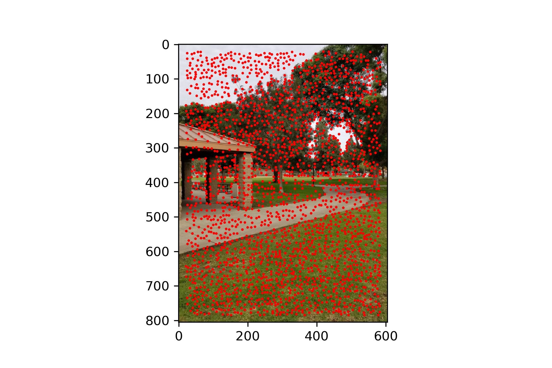
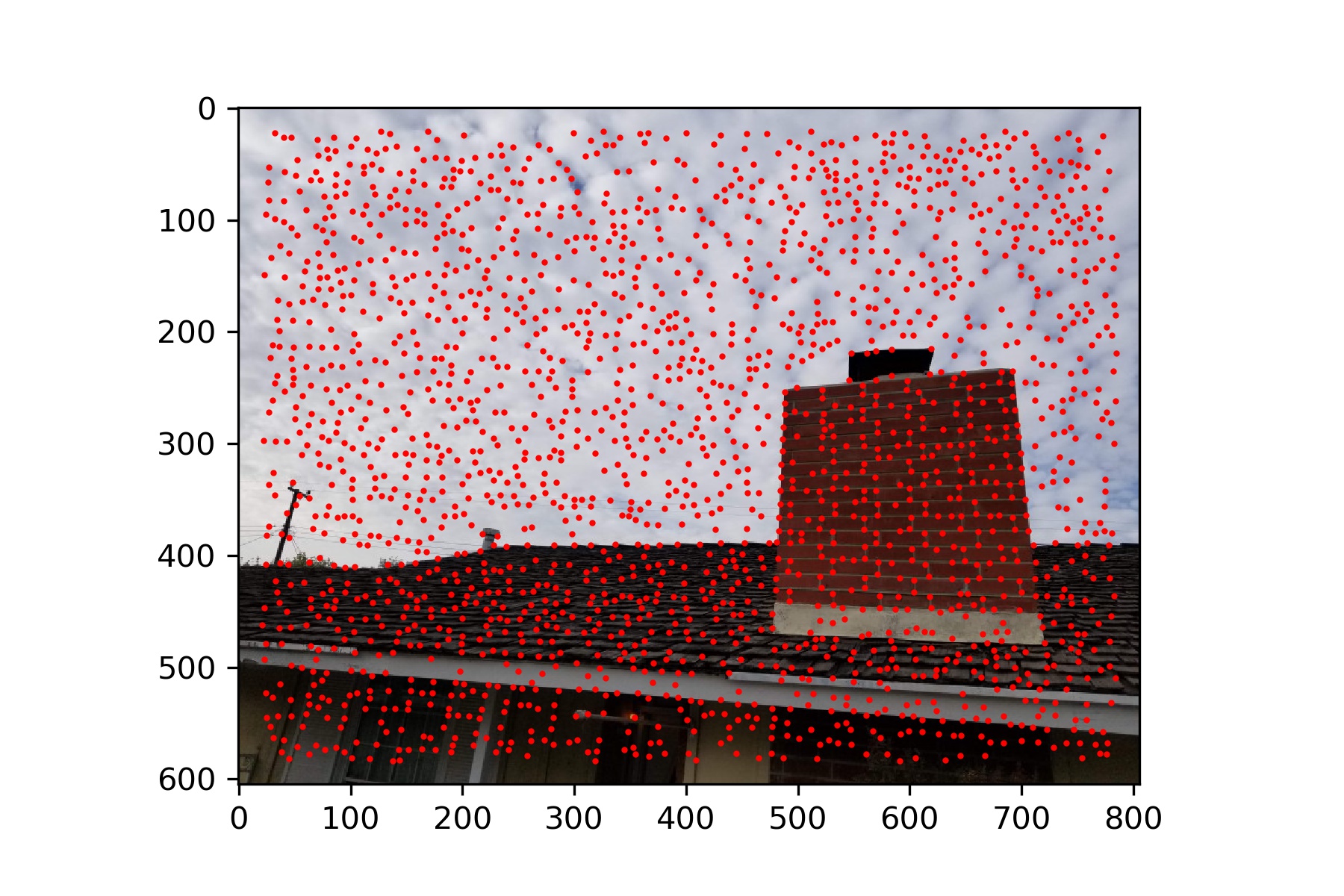
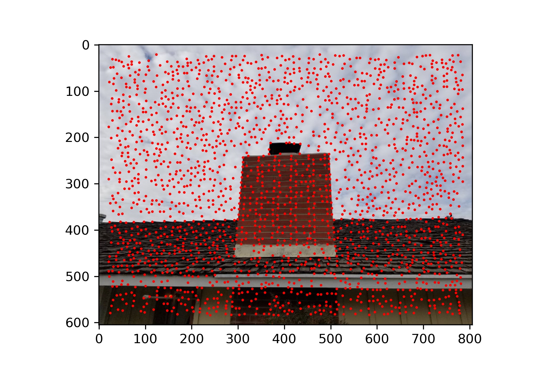
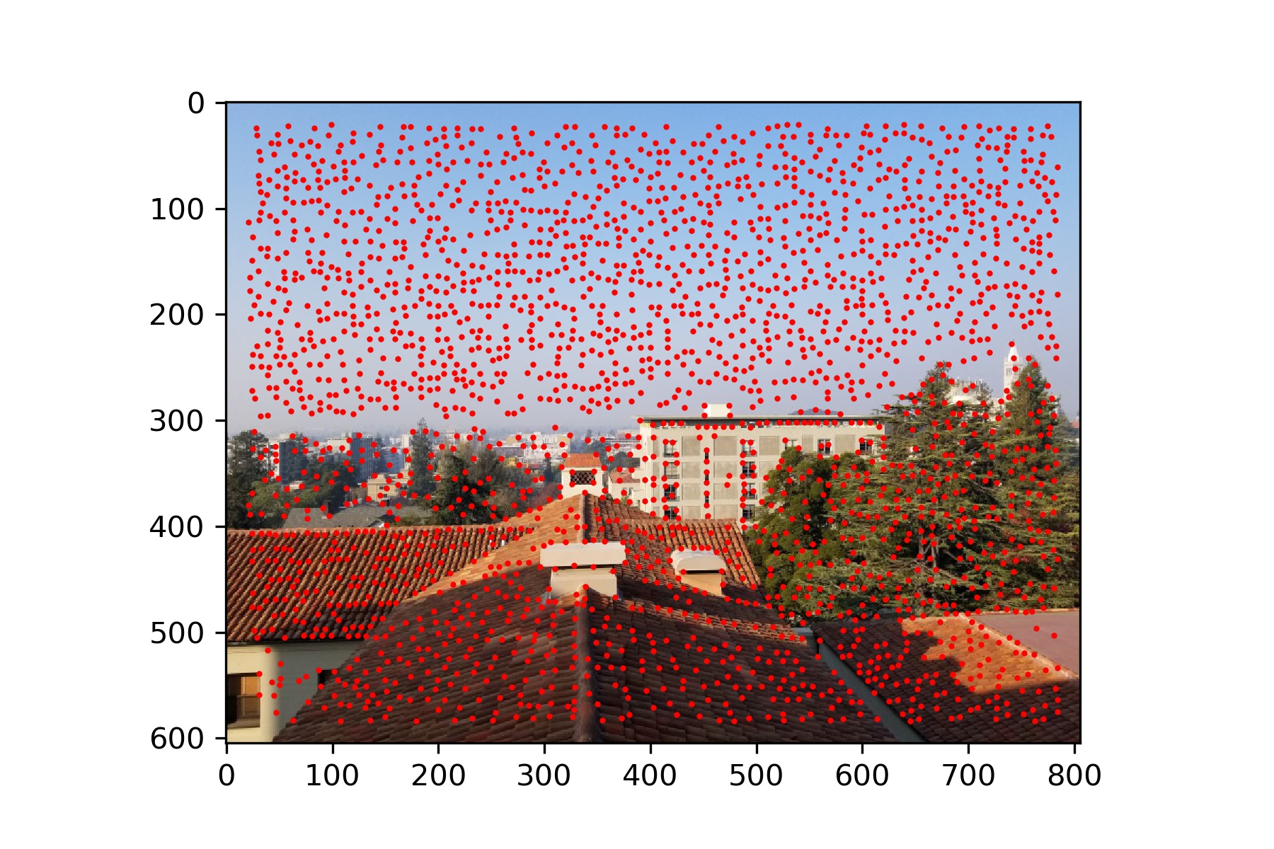
Harris Interest Point Detector
Interest points were generated using the provided function. The minimum distance was changed to 5. The following images show each of the images with the Harris Interest points plotted on top. As we can see, we get a lot of feature points after this step.
|
|
|
|
|
|
|
|
|
Adaptive Non-Maximal Suppression
The goal for this part is to narrow down the interest points, so that we have a specified number of strong points that are dispersed throughout the image. I chose to select 500 points at this step. It is important that we do not just select the highest strength points, because these points may not be well distributed across the image and thus lead to a loss of information. The following images show the remaining points after this step. As we can see, there are fewer points than before but the points still spread across the whole image.
|
|
|
|
|
|
|
|
|
Feature Matching
After finding the interest points in each image, we need to match points between the two images. We do this by first describing features for each interest point. Each feature is a 40x40 pixel square from the image, resized to 8x8. This patch is then normalized so that the average is 0 and the standard deviation is 1. These features give us a way of comparing similarity between regions in the two images. We create a set of features for each image, each centered around one of the points defined previously. Then we calculate the difference between each feature from the first image and each feature from the last image. We consider two features a match if the ratio of one features nearest neighbor over that same features second nearest neighber is less than some threshold value. I set my threshold to 0.4. This checks that the feature must be very similar to its first closest match and also very different than its second closest match. This increases our confidence in the match between the two features. Below show the two images with the locations plotted of all of their matching features.
RANSAC
The last step is to further refine our points through the use of RANSAC. We randomly choose 4 pairs of our matching points and compute the homography. We then apply this homography to every point from our final set of points for our first image and calculate the difference between the resulting point and the matching point from the second image. If this difference is less than some threshold value (I use 5), then we keep this point as an 'inlier'. We repeat this process many times and retain the largest set of inliers. This helps eliminate bad points. The theory is that many of the points should be warped to the correct position by the same homography, and those that are significantly off are not well-matched points. Below are the point correspondences that remain after 200 iterations of RANSAC.
Panoramas
After obtaining a set of point correspondences between the two images, either by manual selection or automatic detection, we use these points to calculate a homography and warp one of the images. After warping the image, I align it to the other image using the position of one of the points from the first image and the warped corresponding point from the second image. From there I blended the images using a weighted average. For each pixel I calculated its distance from the center of that image, weighted the value of the pixel from each image by 1/distance, summed the values and divided by the total of the two scalars. This gives greater weight to those pixels closer to an image's center. As we can see the results do not look good, and this is due mostly to a misalingment. Additionally, better methods of blending could be explored, such as through the use of Laplacian Pyramids.
Results
Rossmoor Park - Manual points
Warped Image
Panorama
Rossmoor Park - Automatic points
Warped Image
Panorama
Panorama without blending
My Roof - Manual points
Warped Image
Panorama
My Roof - Automatic points
Panorama
Warped Image
Berkeley - Manual points
Warped Image
Panorama
Berkeley - Automatic points
Warped Image
Panorama
Conclusion
There is still much work to be done to improve the results, especially with the alignment.
Additionally, the difficulty of this project makes me appreciate the simple panoramic settings on cameras.
|
|
|
|
|
|
|
|
|
|
|
|
|
|
|
|
|
|
|
Conclusion
There is still much work to be done to improve the results, especially with the alignment. Additionally, the difficulty of this project makes me appreciate the simple panoramic settings on cameras.