
Link to 6B: PartB
For shooting the pictures to use for panorams, I made sure to hold my hand very steady and only rotate the camera about its sensor. I also made sure to find areas that had static scenary and easily identifiable corner (such as doors, windows, etc) to make marking correspondences easier.
To recover the homographies, I used a least squares solution to solve for an H matrix that would map im1 points to im2 points and reduce the MSE of im2 points against im2-pts-recovered-from-im1-points.
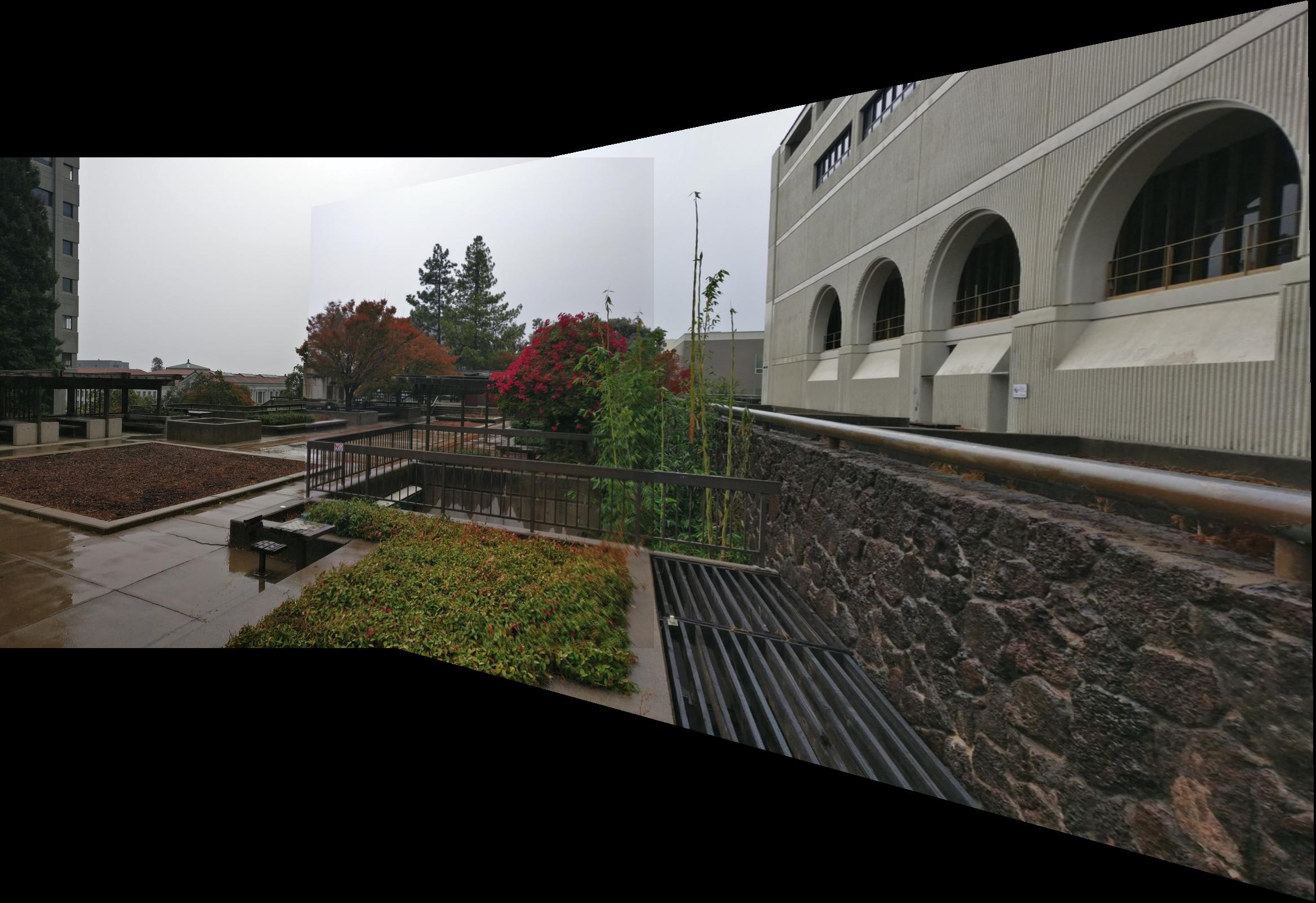
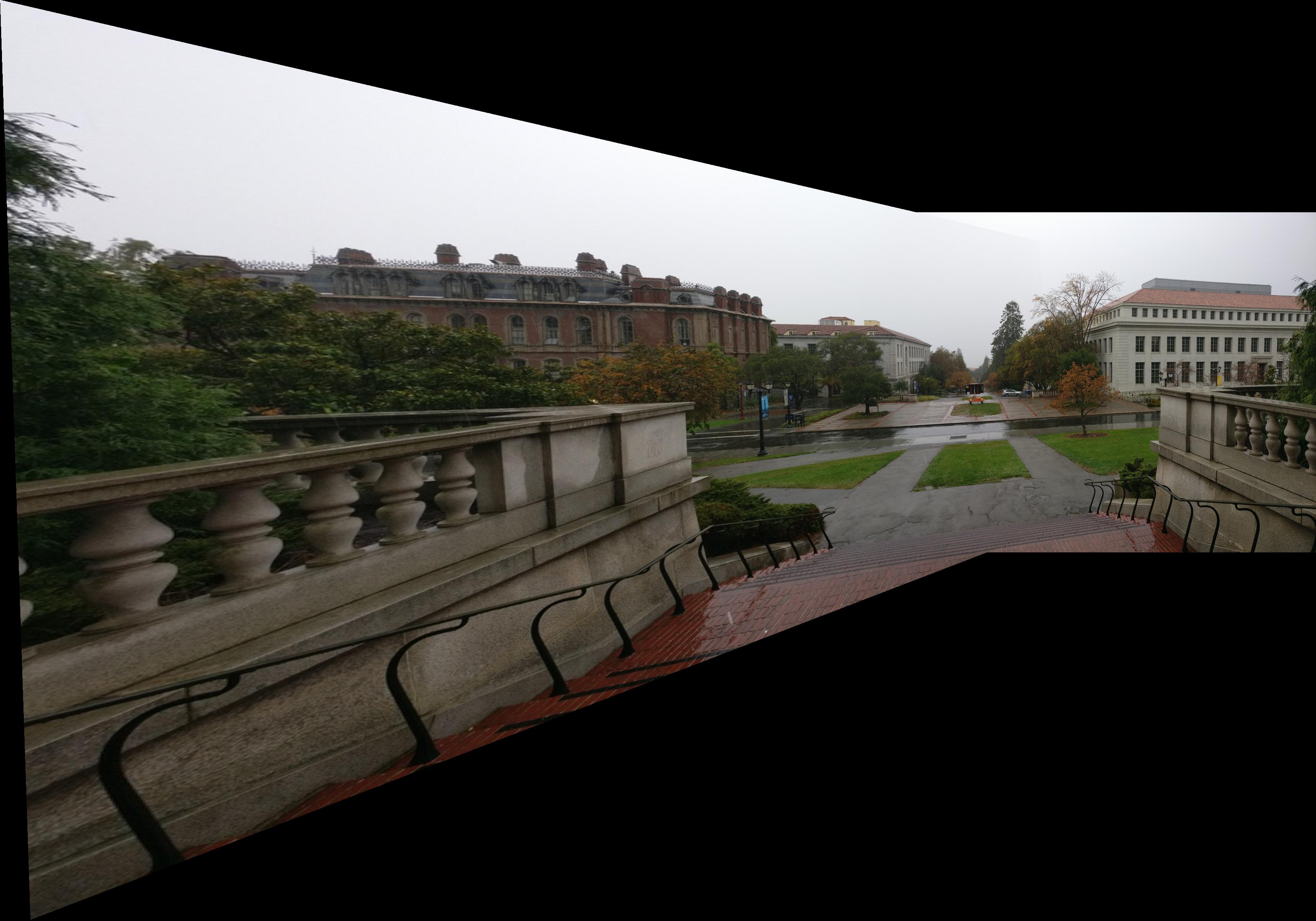
For these operations I used inverse mapping to determine what to do. More specifically I determined the desired size of the final image, be it a rectification or mosaic, and then use the inverse of the homography matrix to determine what point in would correspond to from im1 and the use an interpolation to determine the proper color. Then I overlayed im2 using a similar strategy, but without the homography inverse bit (since the inverse is trivial). Then I used a left to right alpha blending to get rid of image seams, though some seams are still visible.


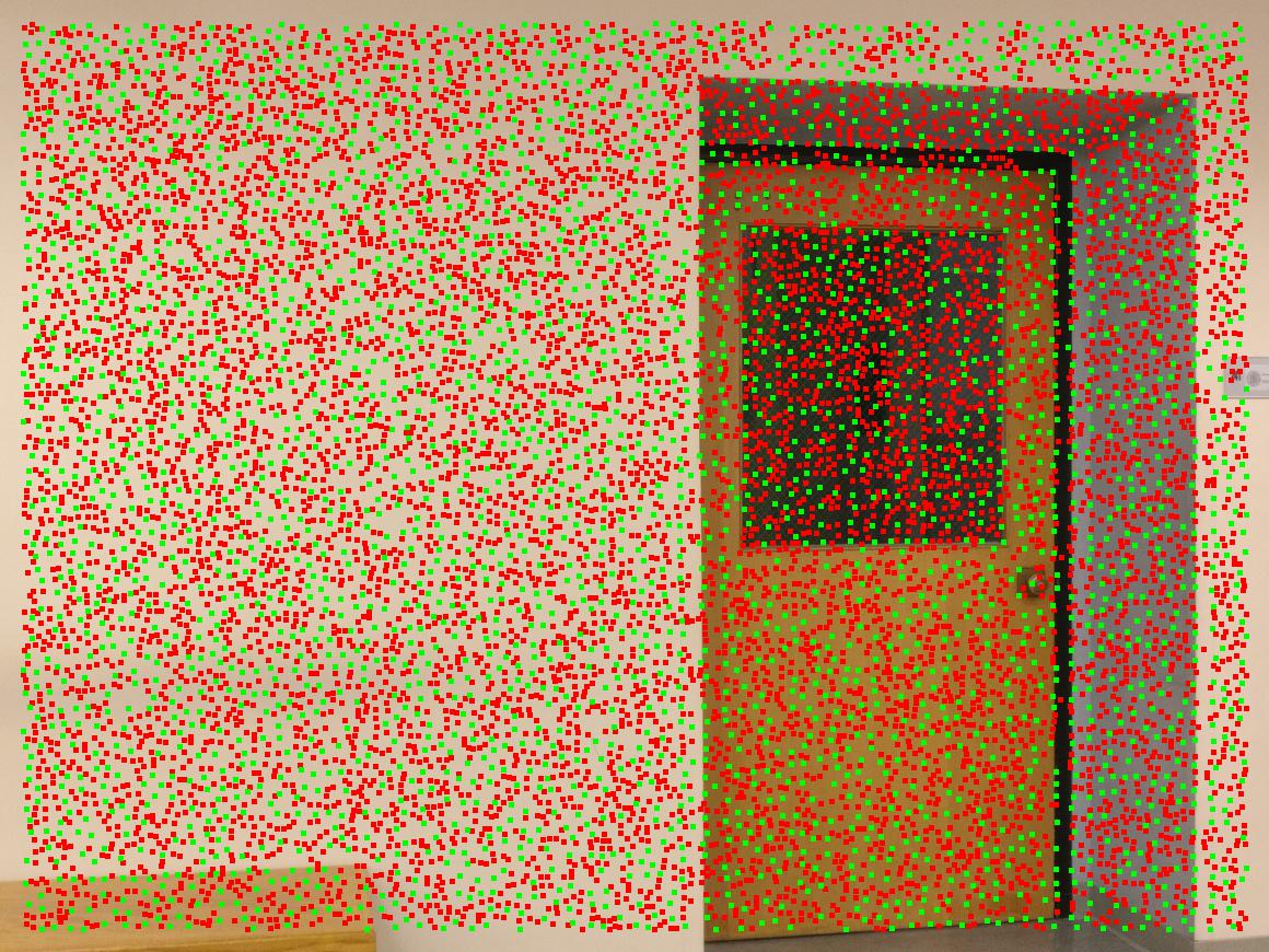
To do this I simply ran the image through the Harris detector. The harris detector gives back a list of interesting coordinates as well as their "intensities". I had to manipulate the minimum distance though, since for larger (high-res) images the detctor will give back way too many interest points.
This algorithm here gets rid of less interesting points as well as triest to remove points in a way such that the remaning "interesting points" are reasonably spread out. I did this by using a nearest neighbor radius search. Given the density of Harris detector I assumed it was safe to say every point had at least 1 neighbor in a 200 pixel radius about it. A point only "survived" if it had the highest interest about a 10 pixel radius. This typically shucked out 80-90% of the points.

For this step I matched interesting points after ANMS from img A to img B. To do this, I sampled about a 40x40 unit square around interesting points in imgA and imgB, downsampled to 8x8 and flattened the matrix. Since instructions where unclear, I tried converting the downsampled images to grayscale and keeping it in color. It doesn't seem to matter in the long run.
Finally we can match interesting points across images. The way this was done was I stuck all descriptors from image B into a 2-nearest-neighbor search where the distance metric was euclidian (which is essentially SSD). Then I took every descriptor in img A and looked at its 2NN in img B. If the closer neighbor's distance divided by the second nearest neighbor's distance was below some threshold, then we had a valid match.
It is interesting to note certain results of feature matching. For instance, in my doors image, it is quite obvious to a human labeller that the easiest feature points to map are the dark corners of the door frame and the recessed frame. However our algorithm refuses to match these. I discovered the reason being is that the right side image has 2 very similar doors, and thus the 2 nearest neighbor distances for one corner of the door is too close (there are 2 very close neighbors since there are 2 very similar door frames) and the algorithm believes the door frame corners to be non-matches, when indeed they are great matches.
I also noticed that in images with reflections on the windows, the algorithm loves labelling those reflections, which is pretty cool since most humans would probably avoid those.
I also noticed the algorithm avoids a lot of obvious corners if they were affected by parallax, which makes sense since those features would be rotated and benerate bad matches.
Finally, to determine which homography to use, I randomly sampled 4 points from the set of matches and calculated a homography between them. Then I mapped all other points in imgA to imgB and saw how many fell close to their correspondensces in imgB. I repeated this 10k times retained the set of points that resulted in the maximal number of inliers. Then, using these inliers, I calcuated a final homography to warp the images together.
I learned some interesting things regarding automatic feature detection and pairing. First, auto feature detection and pairing does not always do "what the humans would do". Even though the algorithm looks for corners and matches them, something humans do when labelling these images, it tends to choose corners in places humans would not. A feature pair that is obvious to a human to be the same point is not so obvious to the algorithm and may be rejected. Furthermore if we look at the differences between human labelled and computer labelled, we see a noticeable difference. Especially in "night", where the computer labelled image maintains the stright line on the railing in the parking lot whereas the human one does not.


