
|

|

|
|
|
|
|
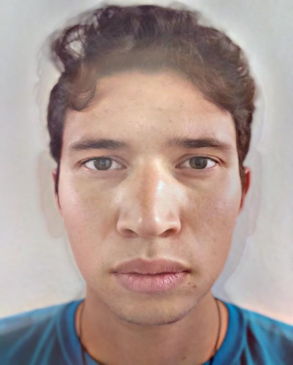
For our final project we take the paper "Style Transfer for Headshot Portraits" by Shih, Paris, Barnes, Freeman, and Durand, and implement it ourselves in Python3. The website for the paper, containing the Matlab implementation and PDF is here. A lot of the techniques used in the paper, such as Laplacian stacks, image warping, and matching, have been learned in this class and used previously, albeit slightly differently. We then take our best implementation of the paper and experiment with its results on our different lighting scenarios. Below, you can find our results in multiple different scenarios.
The goal of this project is to take two photos and transfer one headshot style into the style of another headshot photo. To do this, we warp the stylized portrait into the shape of the other photo, compute the local energy maps, and transfer the local statistics of the portrait into the unstylized photo.
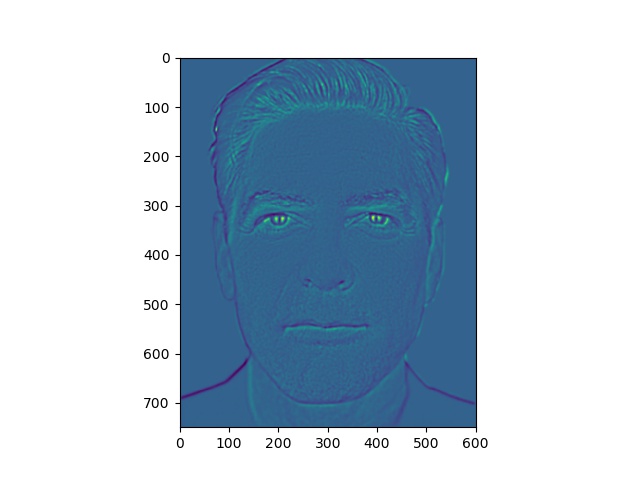
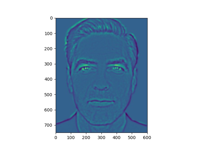
The first step in our process is to compute dense correspondences. Previously, we manually annotated photos to have very exact correspondences. In the first pass of this approach, we attempted to use an automatic software, using dlib and OpenCV, that can be found here. This software finds 66 dense correspondence points specifically in the face region. However, as we explain in our results, the correspondence points only matched the part of the face below the forehead and within the ears, leading to warping issues. Since the Delaunay triangulations were not as exact as in manual correspondences, we resorted to 43 manual correspondences for these specific results, using techniques learned in the face morphing project. From these triangulations, we compute affine transforms and warp one image into the shape of the other. Below are the triangulations found using our manually chosen correspondence points:

|

|
We save our triangulations and points for future use. The next step, according to the paper, is to transfer the local contrast of the image. This local contrast is best seen in the lighting of the image. For example, in the George portrait, most of the light is towards the front of his face. The areas towards the ears and neck are darker.
To transfer the local contrast, we utilize Gaussian and Laplacian stacks. First, we decompose both images into Laplacian stacks, where each level l is defined by this equation found in the paper:

Here, I is our input image, which corresponds to the picture we want to transfer the style to. The input to the Gaussian is a sigma value, and the x is a convolution operator.
We also extract the residual given at stack depth n, defined as

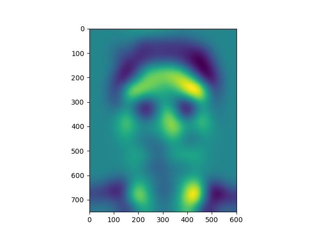
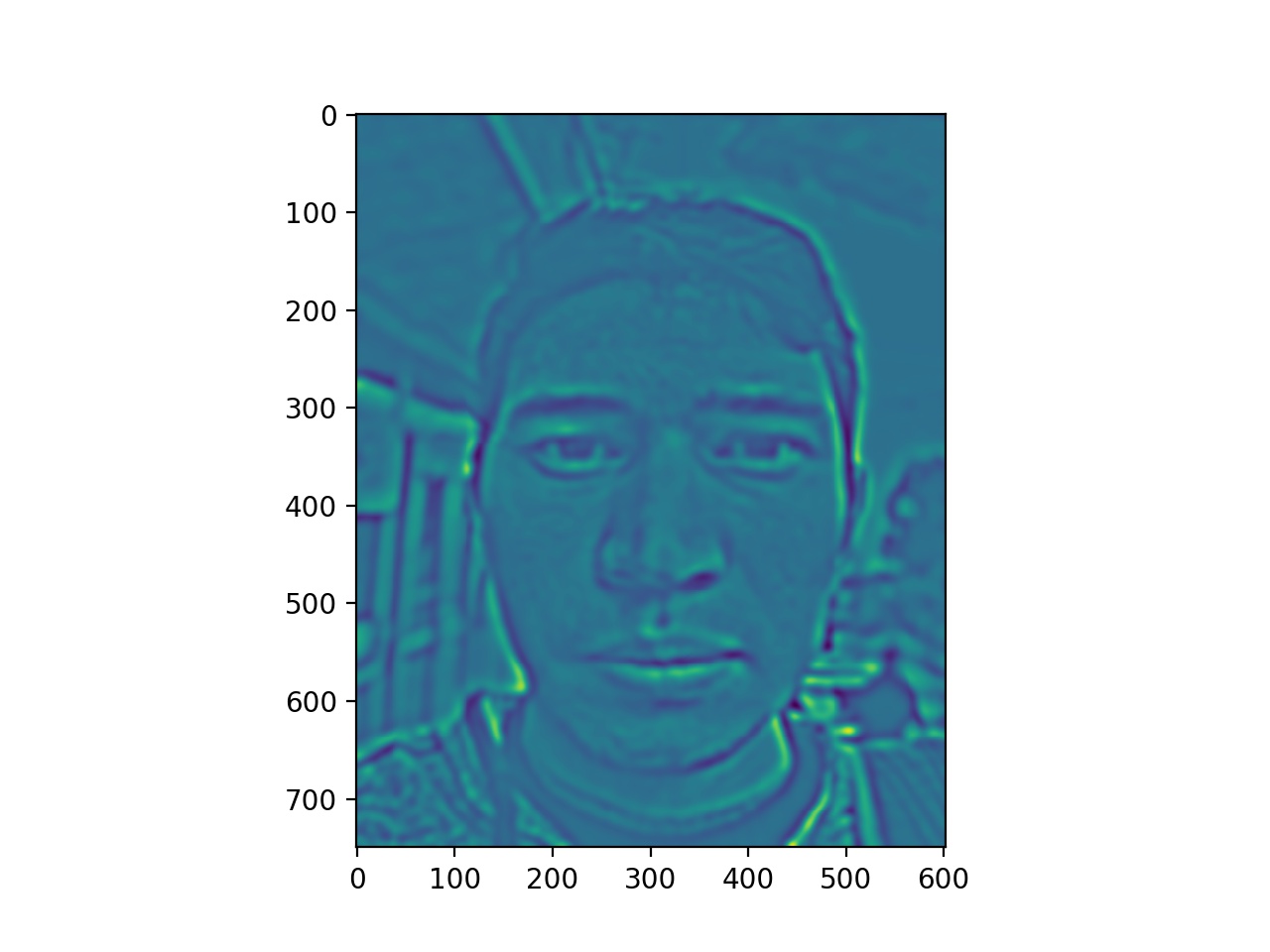
From there, we compute the local energy for both images with the equation below. This step allows us to capture the frequency profiles in the images. As the paper describes, "this estimates how much the signal locally varies at a given scale." Essentially, these energy maps are going to pick up strengths in lighting and color, and they will eventually transfer them onto the image after we sum everything up.
We then warp every level of our portrait energy stack to the shape of our input image, through the triangulation defined in the above section.

At this point, we have energy stacks for both of our images, one for the original image, and one for the portrait warped into the shape of the original. To transfer the energy over, we compute our output as follows, where O is output image of the following operation. S_tilde is our warped example portrait, and epsilon e is a small number to avoid division by 0. In the paper, the recommended value for e was 0.0001:

The square root compensates for the square used to define for the energy.
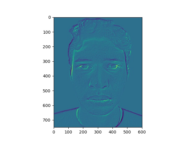
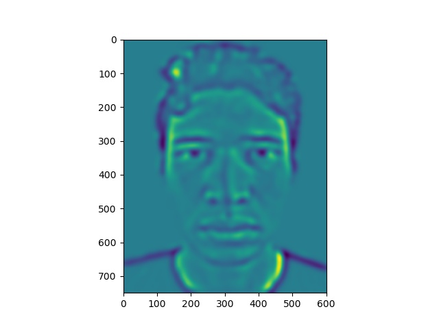
Here, we have some levels of our energy stack images.
Energy stack images for Original Jose picture
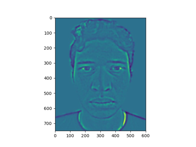
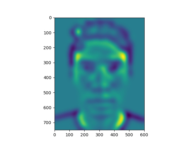
Energy stack images for Clooney picture
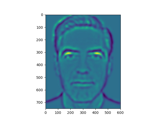
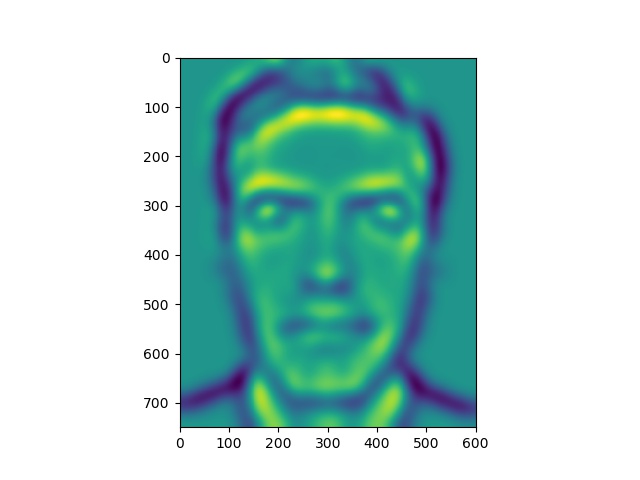
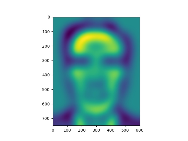
Notice that the yellow areas in the energy maps correspond to most of the light falling on the faces.
Our stacks span 6 levels, the number of levels used in the paper. Also in the paper, the gain maps are clamped to avoid outliers. Explained more in a section below, we clamp the gain at a maximum of 2.8 and a minimum of 0.9 to have robust gain maps. To get our final output image, we warp our example residual into the shape of our original photo and sum up our stack with this warped residual image.
In the paper, the background was directly replaced. In the case that the head size didn't correspond, in which spaces need to be filled with the background, we used the OpenCV method inpaint. What inpaint allowed us to do was to fill in an area equal to the size of the head in the stylized photo, then use that entire image as the background. We first make a mask of the stylized portrait head, then feed the result of removing that area from the whole image into inpaint. The following are the results.


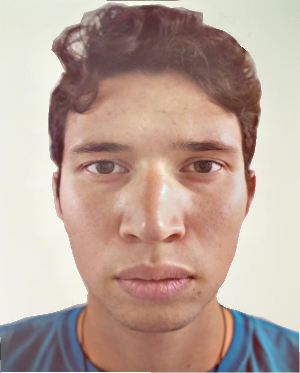
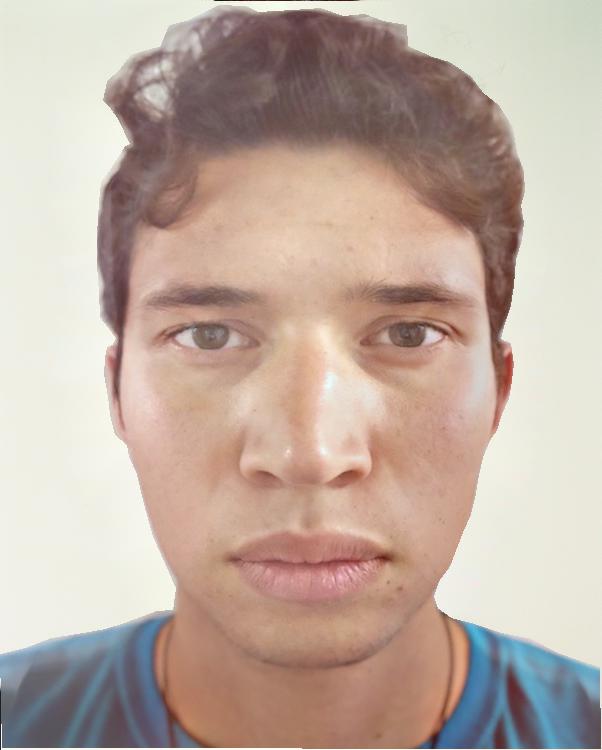
Below, we have the results for transferring the style of Clooney's portrait to the original portrait of Jose. We have original Jose, original George, and transferred Jose. We liked these results, as the lighting becomes balanced throughout Jose's face rather than bright on the right side only. More specifically, the algorithm transfered the lighting focused towards the front of the face. You can see that Jose's forehead is brighter than in the original image. However, the colors are not as bright as in Clooney's portrait, but this can be attributed to Jose's image being much darker to start with and attributed to our robust gain clamping values.

While their implementation did not specify how they defined correspondences, we chose to manually select our correspondences for the George and Jose example. Using the OpenCV automatic correspondence finder, we found that the points did not match regions towards the forehead and outside the ears, so the warped face went beyond our original face, resulting in odd blurs. Below are the comparisons.

The paper had a specific definition for applying a Gaussian convolution to an image. The paper defined it as follows:

We tried this definition but unfortunately we could get this to work. The values outputted by this definition were in a very incompatible range, and our attempts to make it a compatible [0, 1] range failed. Therefore, we continued with regular convolution operations.
Seen in the paper's specific convolution operator, there is a mask. In the paper, a binary mask was drawn over the heads in both pictures, fed into the convolution operator, and applied to the Laplacian layers. Since we were unsuccessful in using the convolution operator above, we only applied the mask to the Laplacian layers. We found that using binary masks gave us different results than not using binary masks. Below, we have our results without a binary face mask and with a binary face mask, respectively. We noticed that not using a mask transfered more of the background/ambient color of the stylized portrait into the face. Not applying the mask to the Laplacian stacks allowed more of the color surrounding the head to be considered for transfer. However, the image now appears too saturated compared to image that did use a mask.

For our experiments, we show the results of using a mask and not using a mask.
The paper demonstrated several examples in which they successfully transfered the style from a black and white portrait to an input image, the final result being in black and white. We tested our algorithm with a portrait of Chris Hemsworth. Then, we repeated the earlier process by finding the manual correspondence points and feeding both images through the algorithm above. Below are the results.

The third image is the result of using NO mask.
From this result, we can see that our implementation was able to transfer lighting directions and areas. For example, in the portrait, the light is strong on the left side of the face, with a dark contrast on the right. In our output picture, the lighting on the left side of the face expanded to a region that matches the lighting found on Chris' left half. Specifically, light can be found on the forehead of the outputted Jose portrait, but not in the original Jose portrait.
However, our result doesn't have the dramatic contrast found in the Chris portrait. Likewise, in the output picture, it appears slightly darker around the chin and along the sides of the face. This, we believe, is because our implemenation managed to treat the facial hair of Chris as a dark spot in the lighting. This is why the upper lip and chin in the output picture appear darker than the light on the left eye. We found this to be an interesting result, as we didn't anticipate the effects of facial hair. This effect was not explained or adjusted for in the paper.
To address the lack of dramatic contrast, we experimented with the clamping values. The results will be displayed in a further section. Below are the results with a mask.
The third image is the result of using a mask.
In this section, we dicuss our observation with clamping gain values. According to the paper, "gain values below 1 mean a decrease of local contrast, and conversely, values greater than 1 mean an increase." The paper defines a robust gain map that clamps high and low values:

The paper defines theta_h = 2.8, theta_l = 0.9, Beta = 3
Values were clamped to avoid "phantom" effects. Our clamping was done very fast by vectorizing our code.

Notice that there is a convolution with a Gaussian at the end of clamping. The results we have obtained so far didn't use this convolution operator. This is because, when looking up the Matlab implementation found the paper's website, the code's implementation actually didn't include this convolution. Thus, we didn't technically include this descision as a deviation. However, we ran some tests using this convolution operator.
Below is the result of including the convolution at the end of clamping.
The third image is the result of applying a Gaussian convolution at the end of clamping.
Comparing both pictures.
The convolution at the end of clamping produced the right picture.
We found the convolution at the end of clamping to be less dramatic. For the rest of the results, we didn't include this final convolution operator.
Using the intuition mentioned earlier, we experimented adjusting these clamping values. For the Jose and George picture, we tried to increase the contrast of the light by increasing the min and max gain values. Below is the result of a min gain of 1.1 and a max gain of 3.0:
The image on the right has a theta_h = 3.0, theta_l = 1.1.
To us, this was surprising. We expected the contrast to be better, since by increasing the min gain to be above 1 made us think that the lighting would be more dramatic. With the higher min and max gain values, a lot of the lighting transfer is gone. So since increasing the min gain didn't help, we tried decreasing the min gain back to 0.9. Below is the comparison.
The image on the right has a theta_h = 3.0, theta_l = 0.9.
Now we noticed no difference between the result with the higher max gain and the default max gain. After this, we decided to lower both numbers to 1.7 and 0.5:
The image on the right has a theta_h = 1.7, theta_l = 0.5.
Lowering both the min gain and the max gain made the output image significantly more washed out. This result confused us because it seemed to go against the intuition that the paper mentioned, in which we expected that the higher values would make the lighting more dramatic. In addition, when we lowered the values, the image color was completely washed out. We unfortunately weren't able to come up with an explanation for these results and didn't find any useful information on this in the paper. For the rest of the project, we kept the min and max gain values as the default ones from the paper.
The main goal of implementing this paper was to experiement transferring portrait styles from non-studio lighting scenarios. That is, in the paper and so far for this project, we have looked at transferring styles from a very stylized portrait, likely taken in an indoor studio with fancy lighting equipment. We came up with a new question: can we transfer styles from an indoor setting to an outdoor portrait and vice versa? Essentially, we tested our style transfer with non-stylized portraits and focused on natural environments. We aim to show the results, then discuss what transfered well and what didn't transfer well.
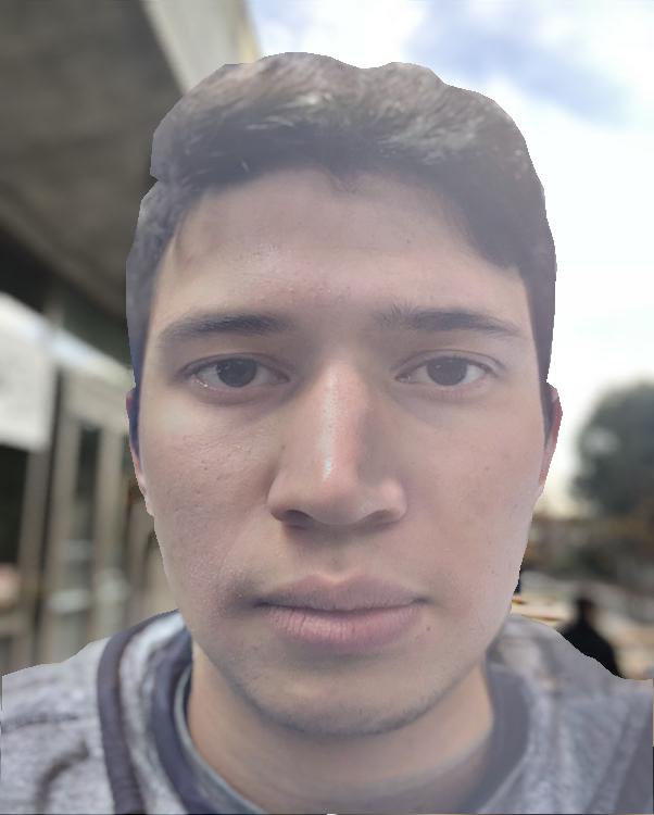
Below are two portraits in natural environments, one indoors and one outdoors respectively.

|

|
The algorithm used for the experiments below uses manual correspondence finding and default clamping values.
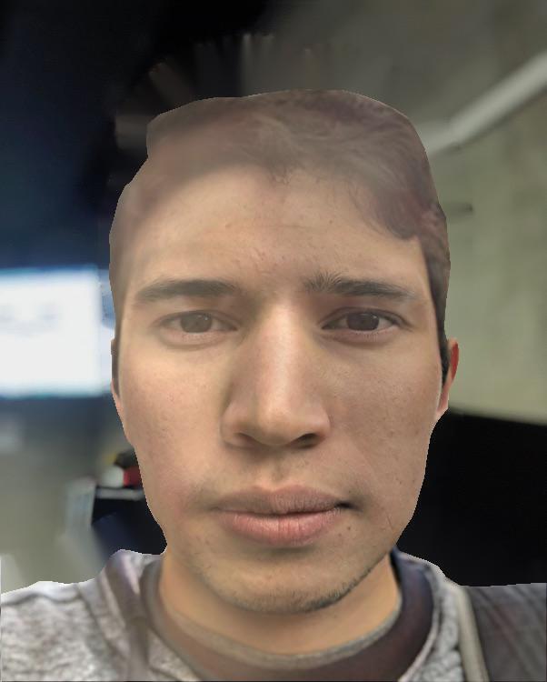
We tested transferring the style of the outdoor portrait to the indoor portrait, replacing the background. Below are the results.


The third image is the result of using a mask.
The third image is the result of using NO mask.
As before, our algorithm managed to transfer the very diffused lighting found outdoors to the face in the indoor picture. However, now our result looks too washed out. We believed this was a result of our algorithm's deviation from not blurring the mask in the laplacian stacks, which would have helped transfer more matching color values surrounding the head.
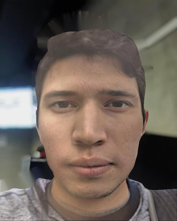
Here are results from going from outdoor to indoor.
The third image is the result of using a mask.
The third image is the result of using NO mask.
Overall, much of the very diffused outdoor lighting on the original outdoor image was replaced with the lighting found in the indoor picture. If you look closely, the right side of the face in the output picture matches the lighting of the original indoor picture. The result obtained from not using a mask had better color matching than the results obtained using a mask.
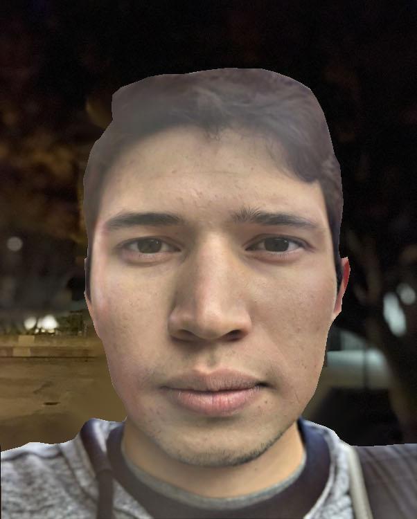
We also tried going from outdoor lighting to night lighting.

The third image is the result of using a mask.
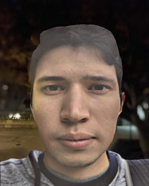
The third image is the result of using NO mask.
In general, the outdoor to night lighting experiment failed. One positive aspect is, in the result with no mask, the yellow highlight on the right side of the faces was transferred. But, our algorithm does not transfer color as well as local contrast.
Another combination is from night to daytime lighting.
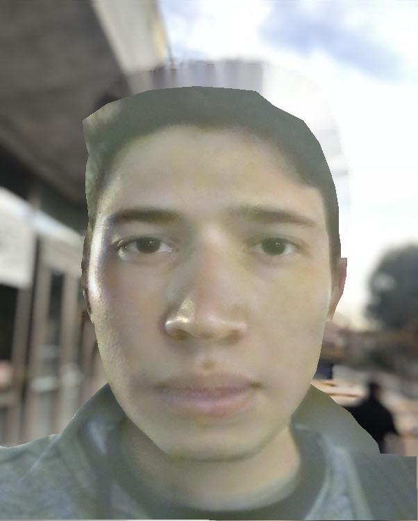
The third image is the result of using a mask.
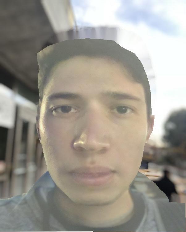
The third image is the result of using NO mask.
In general, a lot of our color could not be transfered like they were transfered in the paper. Taking into account implementation differences, we couldn't develop an explanation as to why we couldn't transfer color effectively. At this point, we thought that the differences in our implementation, such as the masked blurring, manual correspondence points, affected the transfer of color. In the next section, we show the results of us using auto correspondence finding rather than manually found correspondence points.
Our more promising result from the indoor outdoor experiments came from using the OpenCV/dlib program mentioned earlier that automatically found dense correspondence points on the faces. Below is the comparison of the results of going from indoor to outdoor.
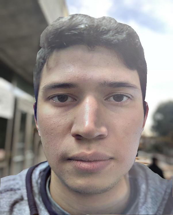
The image on the right was obtained using automatically found correspondence points by the OpenCV program and a mask
The image on the right was obtained using automatically found correspondence points by the OpenCV program and NO mask
To better analyze the difference, we looked at the warped energy stacks. The images on the right are the images found using automatically found correspondence points and the images on the left are the images found using manually found correspondence points.
Already we noticed that the warped energy stacks with manually found points have more overall energy in the picture, producing an overall greener tone versus the photos with the automatically found points, having less overall image energy. Everything up to this point in the algorithm has remained the same for both automatically and manually found correspondence points. Therefore, having those manually found correspondence points led to an overall energy increase.
One possible explanation for this is that the 66 points found using the automatic program increased the density of the triangulation in the face region, therefore making the triangles smaller. Taking into account that the faces are relatively positioned similarily in both photos, most of the triangles didn't have a large warp, which would have led to heavy color interpolated. Instead, the small warp values meant that a lot of the original color was more accurately transfered over. The less dense manually found points introduced the possibility of larger warps as the triangles were larger.
Overall, the color transfer worked better for this example, especially since we used Jose's face in both images, roughly the same size in each image. Recall that this didn't work with George's head which was significantly bigger in his portrait.
The best results came from automatically finding dense correspondence points and not using a mask on portraits with similar head sizes and positions. For transferring styles between different head sizes, manually finding dense correspondence points worked to avoid "ghost" effects. In addition, the default clamping values in the paper allowed for the best contrast as our own attempts to increase the contrasts failed.
We enjoyed this project as we got to learn about energy and gain maps and how they work to transfer lighting and color. It refined our knowledge of warping, Laplacian stacks, and using correspondences. Finally, we were able to output a few decent results, such as the George-Jose result and the indoor to outdoor result with automatic correspondences. We unfortunately were not able to accurately explain some of the results with testing different clamping values, but tried our best in explaining how choosing to automatically find correspondence points led to better color transfers.