CS194-26 Project 1 - Eric Leong
Background
Sergei Mikhailovich Prokudin-Gorskii (1863-1944) traveled throughout the Russian Empire, taking colored pictures of all kinds of things. To taking colored photos, he took three exposures of every scene onto a glass plate using a red, a green, and a blue filter. These RGB glass plate negatives survived and were purchased by the Library of Congress, and were recently digitized, becoming available online. In this project, we used the digitized RGB glass plate negatives to produce accurate, vivid, colored images.
General Approach
My approach to formulating colored images from the RGB color channel images followed the steps in the starter code, which was to first read in the image containing 3 separate color channels and splice image into 3, so that we can extract each of the 3 channels: R, G, B. For Bells and Whistles, I added an additional step for auto-cropping the borders of the image, using the Scharr edge detection technique on each of the channels and selecting the crop that reduced the image size the most. Auto cropping added 2 additional parameters: threshold, and max border where threshold determined the sensitivity of what we considered a border and max border determined the highest proportion of the image side we'd crop. For instance, .1 max_border would mean we would at most crop 10% from the left, right, top, and bottom. The next step was to align the red and green channels to the blue channel accurately. I used 2 approaches for finding the best alignments: exhaustive search and image pyramid. After the best alignments were found, I adjust the channels accordingly and finally stacked the channels to produce a colored RGB image.
Naive Exhaustive Search Alignment
The exhaustive search algorithm, implemented in align(), takes an image channel as input and outputs the best alignment on both axes x, y. I performed exhaustive search in the range [-15, 15] for x and y, displacing the red channel image and green channel image in every possible combination of x, y values within the range and comparing each displacement to the unadjusted blue color channel image. To compare the images numerically, I computed the SSD (sum of squared differences) value between them, and ultimately selected the best displacement values by choosing the one that had the lowest SSD. I also tried computing the NCC but I did not notice any change in the result, so I stuck with using the SSD. The exhaustive approach was very slow for the larger .tiff images, taking over 10 minutes to run for each, making this alignment approach impractical.
Image Pyramid Alignment
Because the exhaustive search approach was extremely slow, I implemented the image pyramid algorithm. The algorithm similarly takes as input one channel image to perform the alignment on, along with a scale factor. The scale factor determines the number of levels, which we compute in the beginning based on scale factor and the input image size, as well as the difference in scale between each level. For instance, the 2nd highest level will be have dimensions: base * first level dimension. To improve speed, we set the cap of the number of levels to 8, since rescaling images to significantly smaller scales served to be a bottleneck. Each "pyramid" level consists of a rescaled version of the input image, and is based on the scale factor and an exponent. The exponent ranges from 0 to the capped number of levels as can be interpreted as the magnitude of the rescaling factor, where if the exponent is higher, the image is smaller.
To perform image pyramid alignment, we start from the smallest pyramid, which is when the level is highest/ image is smallest and perform the naive exhaustive search to find the best alignment/offset at that scale. Once we find the best offset at the scale, we move onto the next level, where the image size will be base * previous and we again perform the naive exhaustive search but with a smaller adjusted range, centered on offset * base, to find the optimal offset at the level. We repeat this process until we have the optimal offset of the image at the original resolution, when exponent = 0.
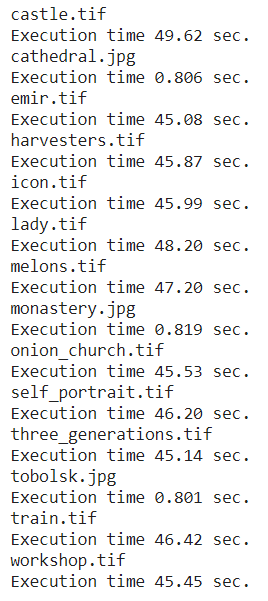
To get the results, I used a scale factor of 2 for each of the images, and set the max number of levels to 8. This led to an execution time of around 1s for the smaller non-tiff images, and a time of around 45s for the large tiff images. This could be seen in the following image:
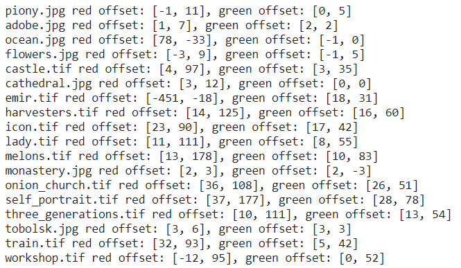
These are the resulting offsets computed for each image.
Results using Example Images
castle.tiff
cathedral.jpg
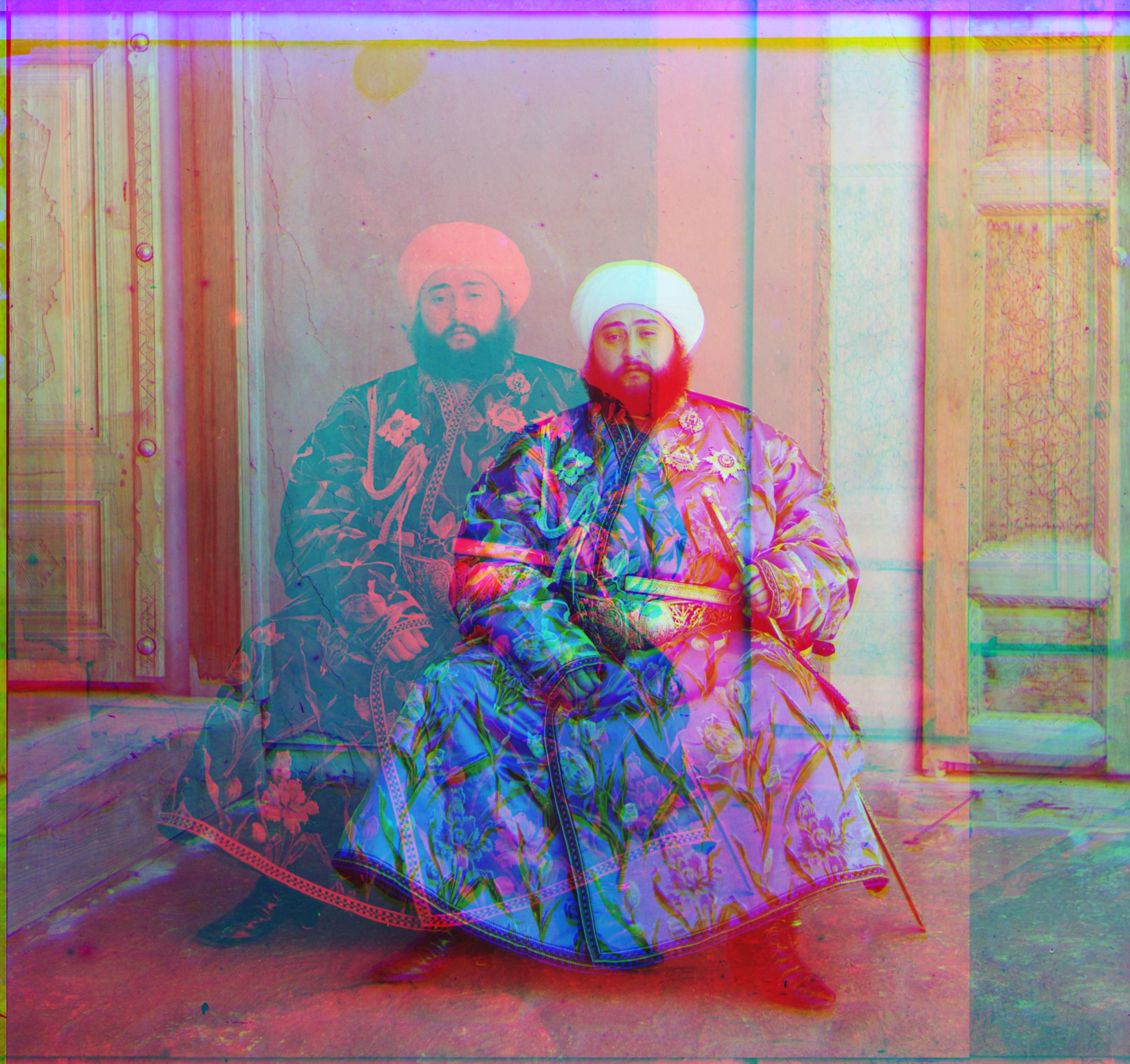
emir.tiff
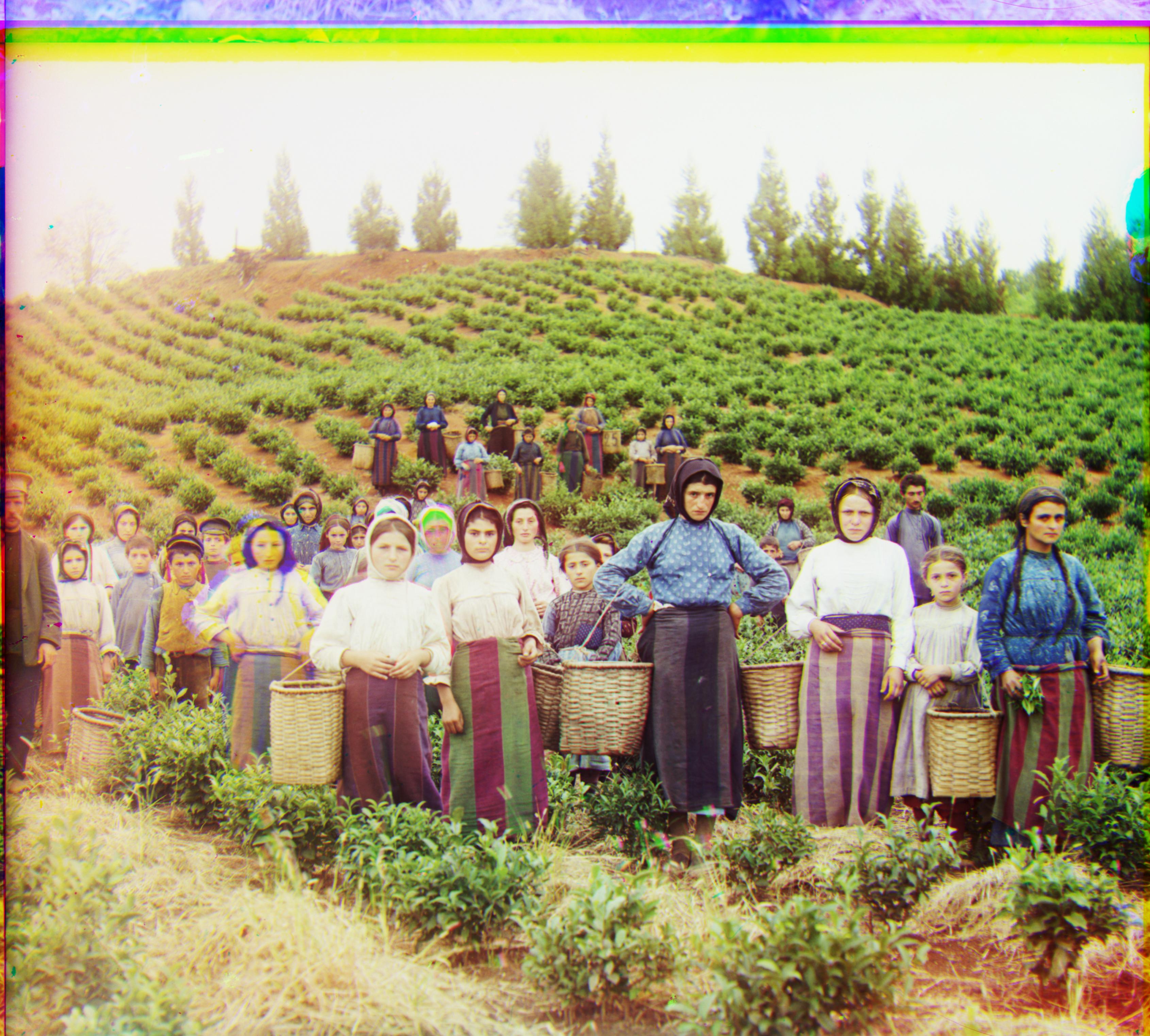
harvesters.tiff
icon.tiff
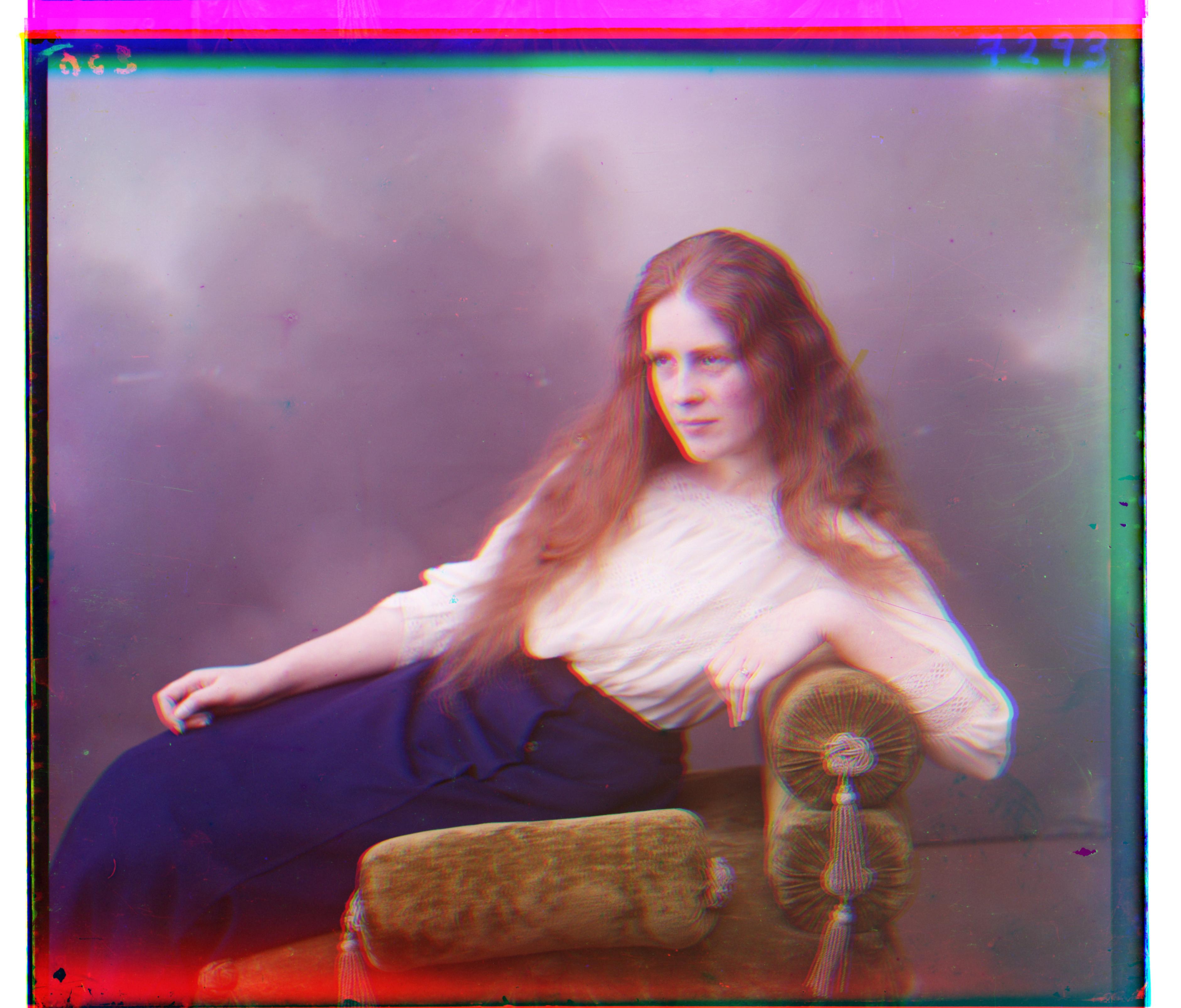
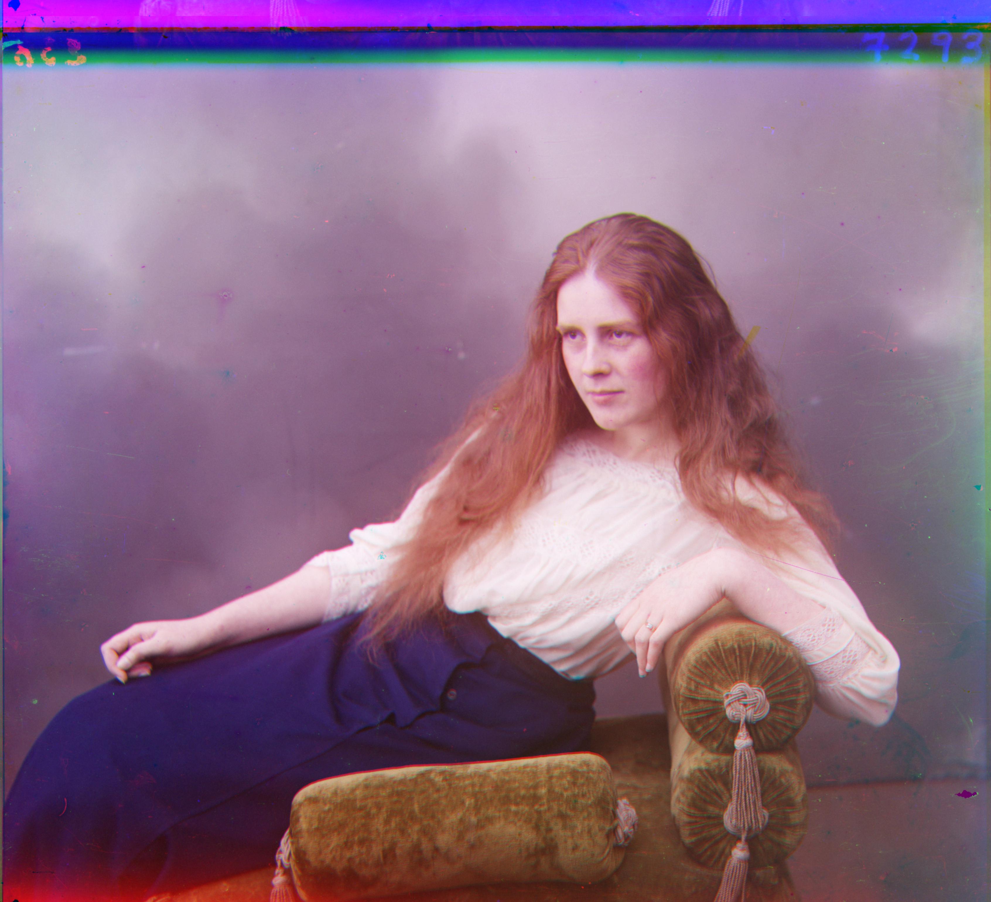
lady.tiff
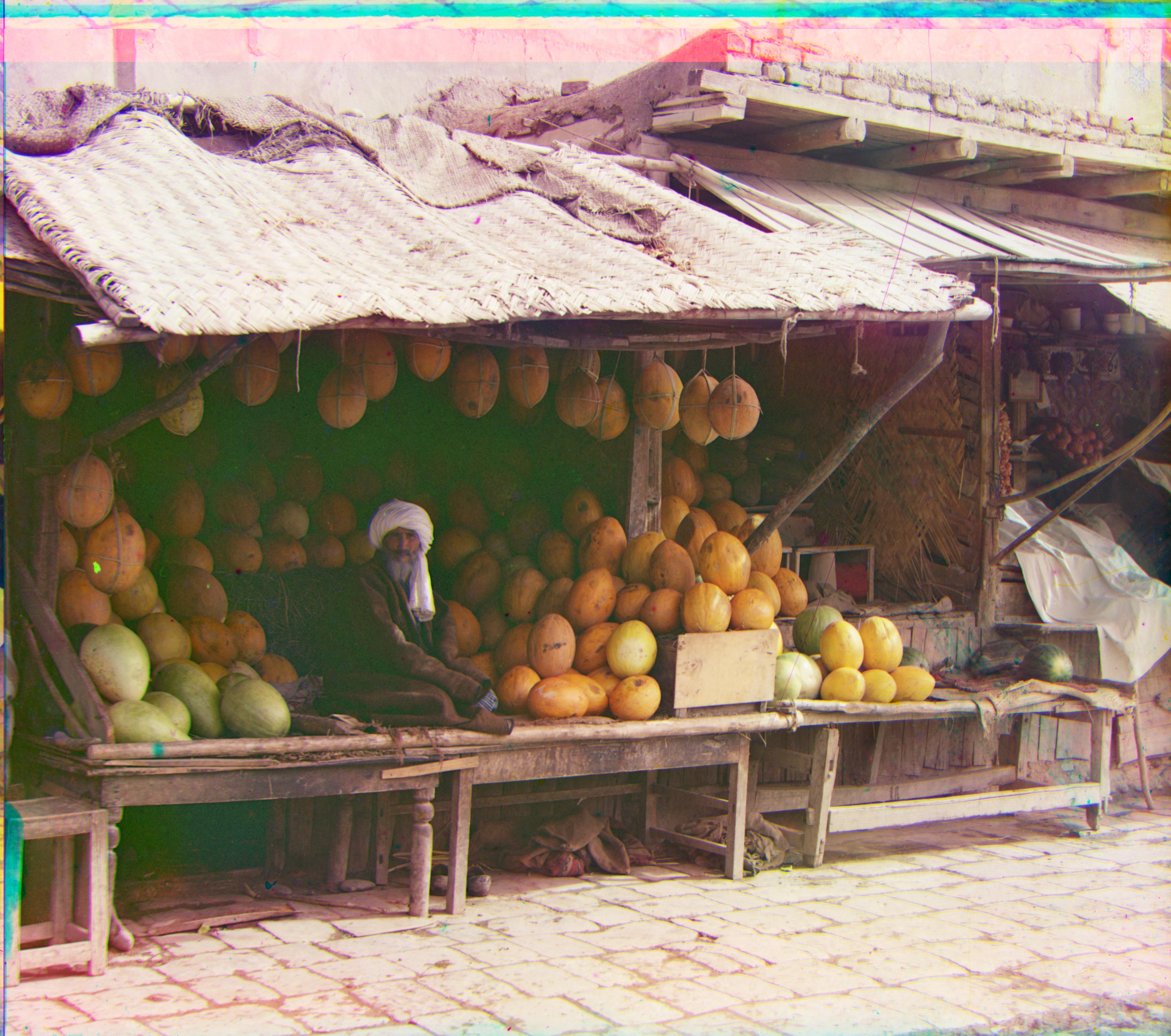
melons.tiff
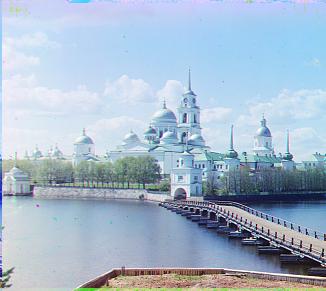
monastery.jpg
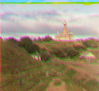
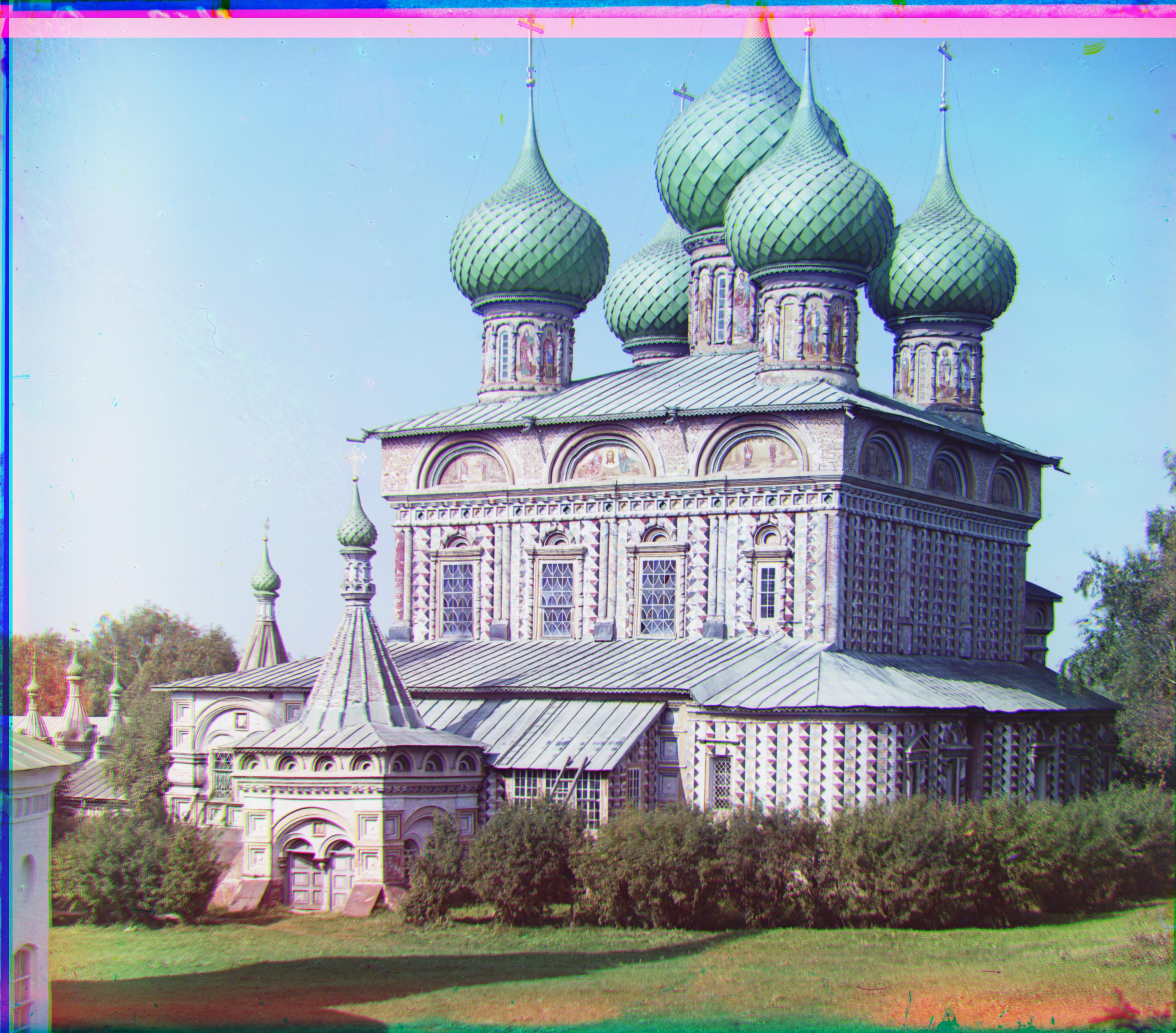
onion_church.tiff
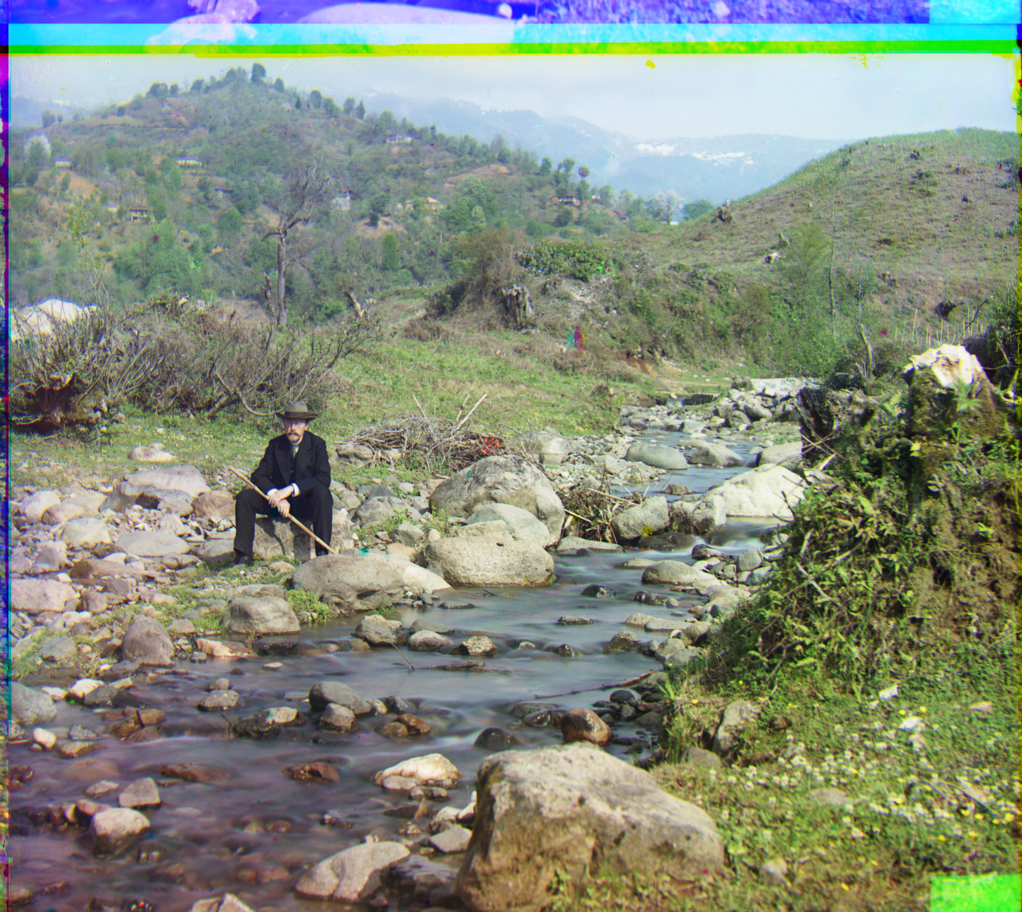
self_portrait.tiff
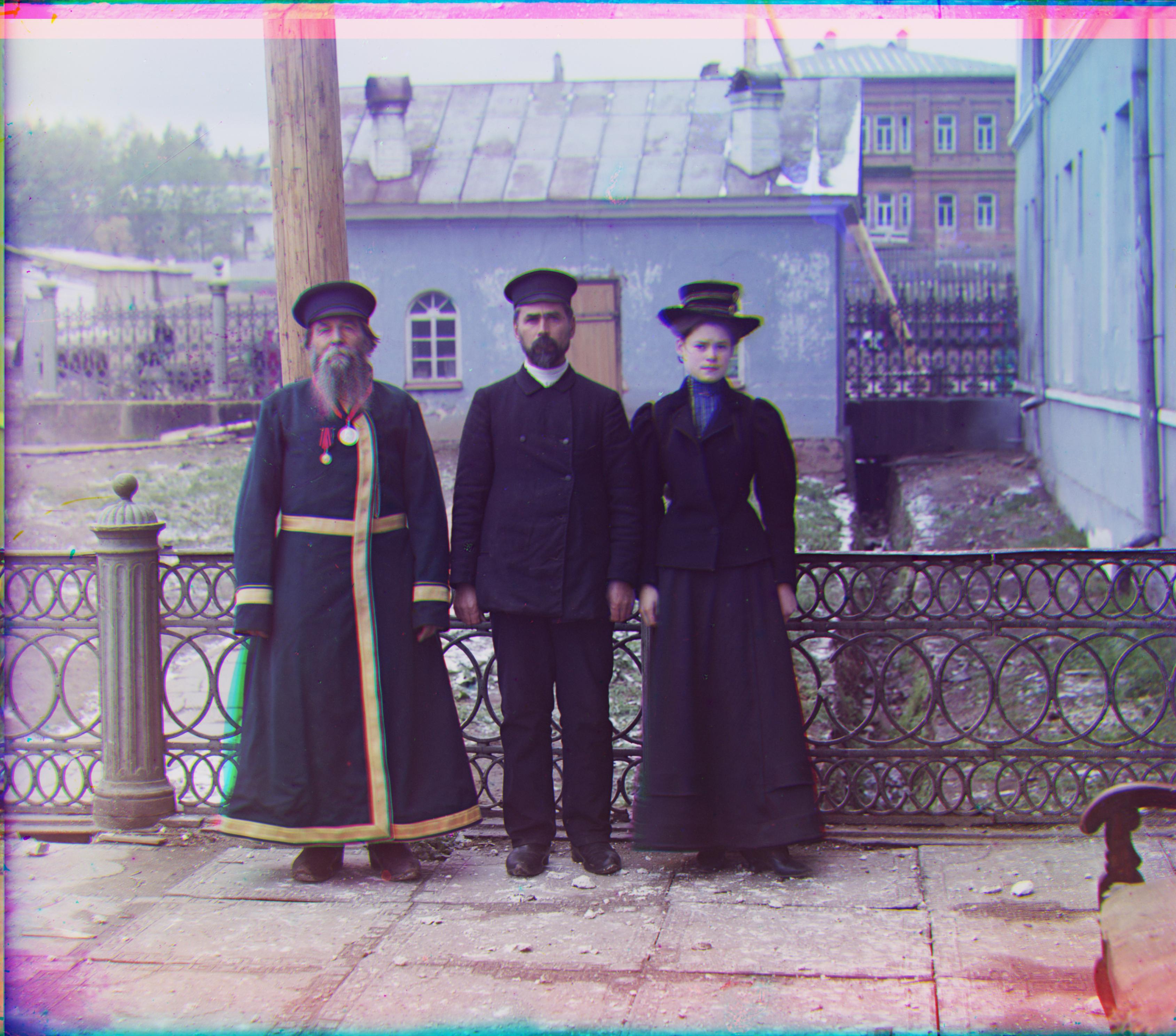
three_generations.tiff
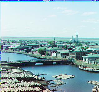
tobolsk.jpg
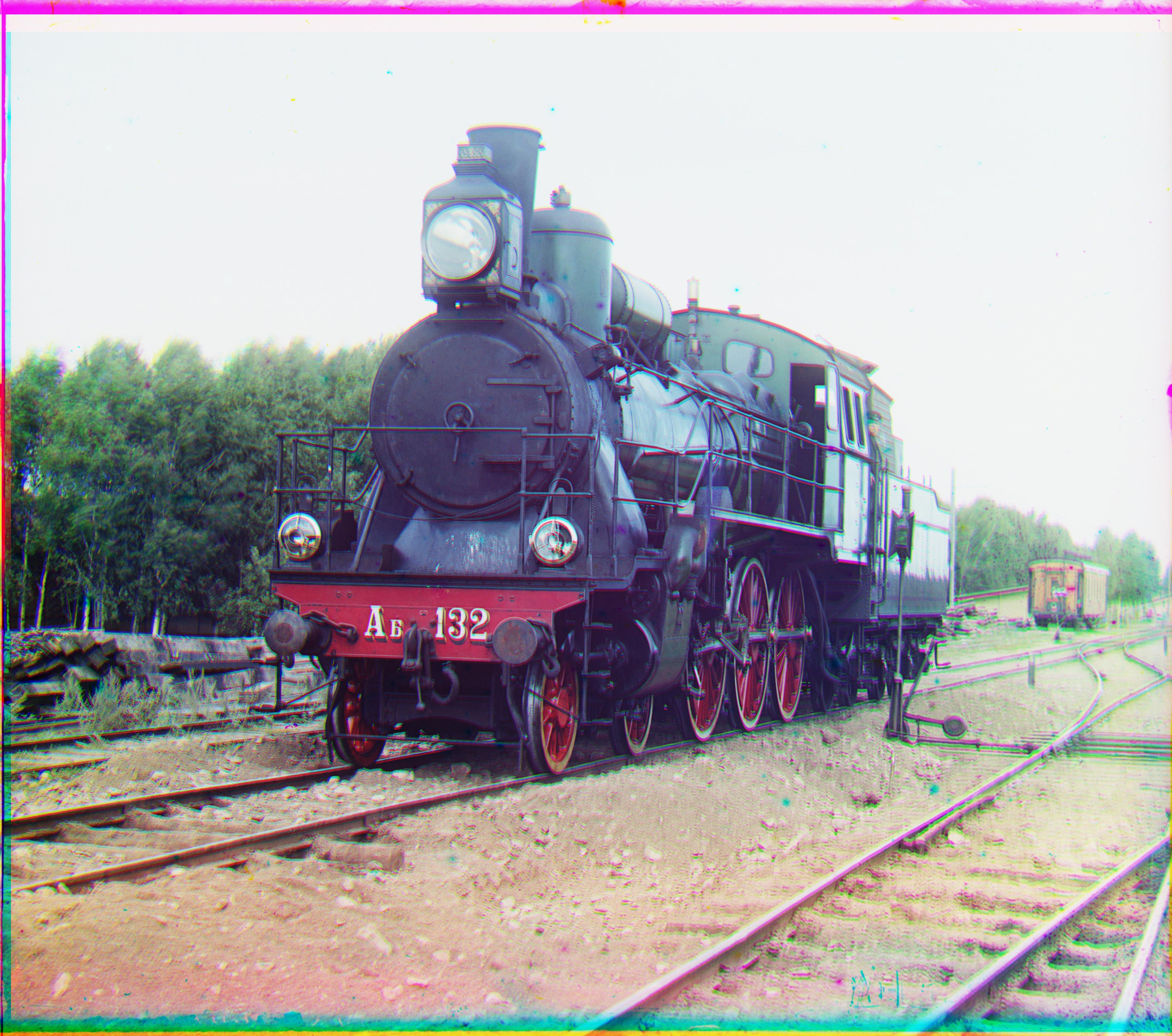
train.tiff
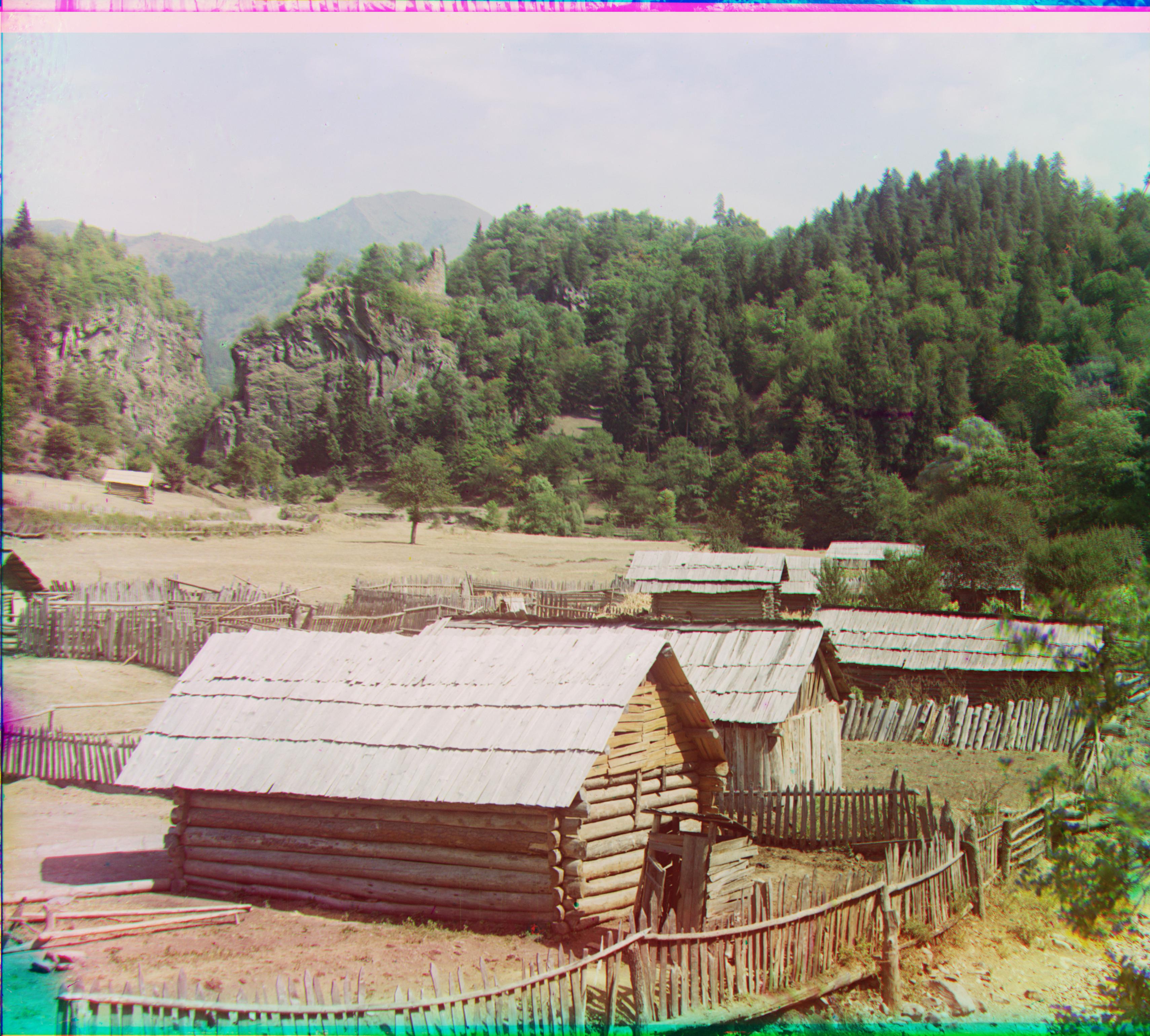
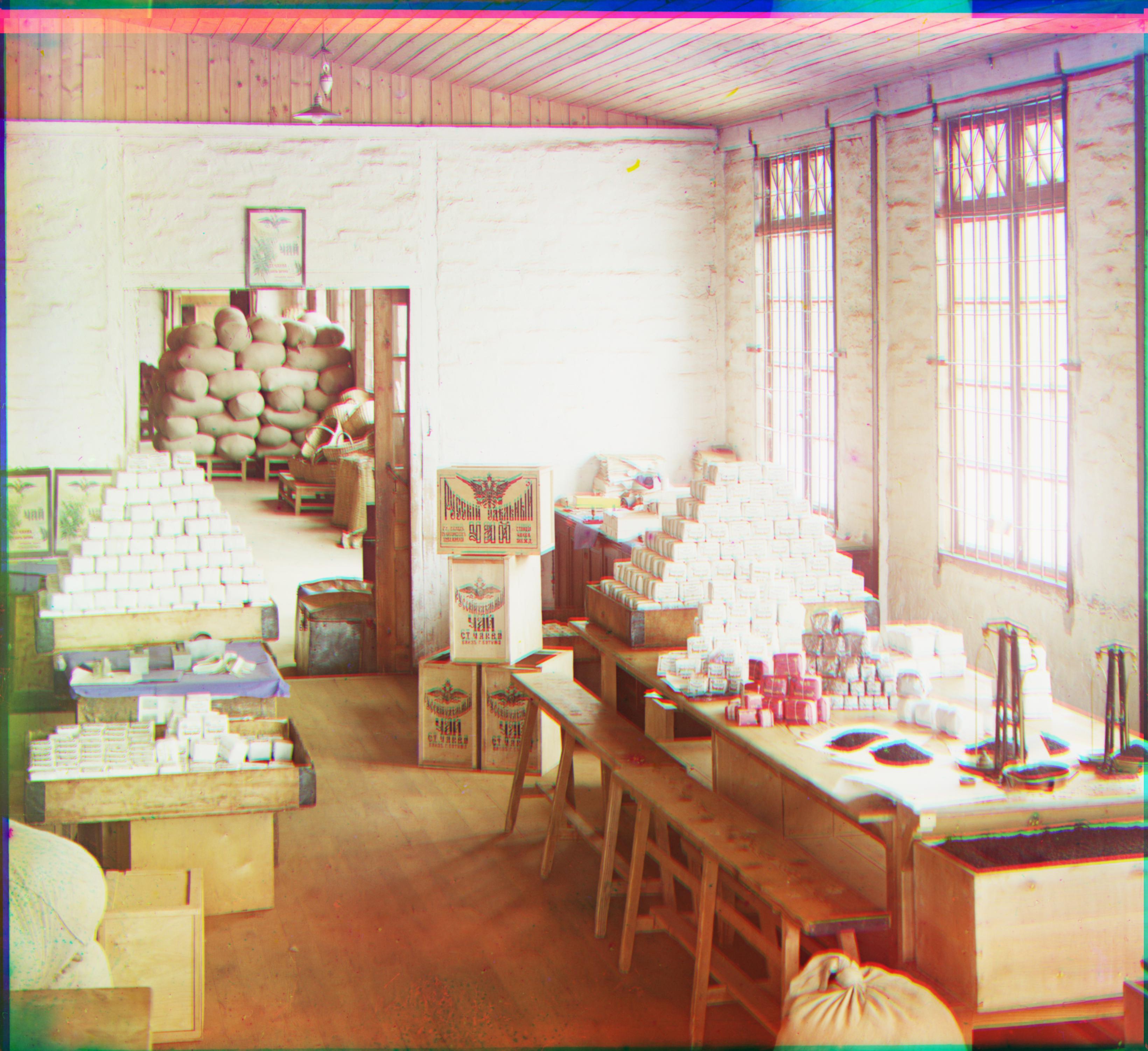
workshop.tiff
Results on Selected Images
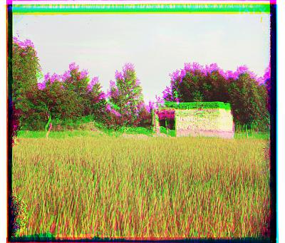
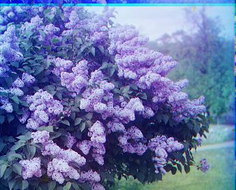
flowers.jpg
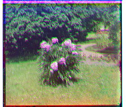
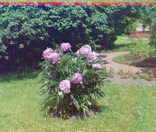
piony.jpg
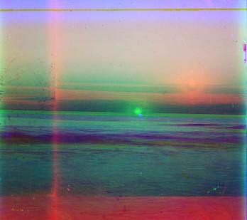
ocean.jpg
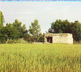
adobe.jpg
Bells and Whistles
Auto Cropping using Scharr Edge Detection
As mentioned in the General Approach section, I performed auto cropping before computing the optimal alignments of each of the channels. I created 2 helper functions: auto_crop, which performed the auto crop procedure and outputted indices t, b, l, r such that the cropped image would be im[t:b, l:r], and border_index, which computes the index for a specified side of the image. In auto_crop, we first apply the edge detection filter with a Scharr operator. There are other operators, such as Roberts, Sobel, and Laplace, but I was not able to determine which worked best. After applying the filter, border_index is called in where we go column by column (or row by row) starting at max_border, computing the sum column and checking if it meets the specified threshold. We repeat this for all sides of the image, which leads to the output. Cropping the image using edge detection to detect the borders was successful, and it removed the noise that the borders created, making the alignment process more accurate. Some examples where auto cropping improved the final image are shown, where the left are images without cropping and the right includes images with auto-cropping.