In the early 1900s, Sergei Mikhailovich Prokudin-Gorskii traveled across the Russian Empire and took numerous colored picture with his simple but genius idea. He record three exposures of every scene onto a glass plate using a red, a green, and a blue filter. However, the techniques back then was unable to recover the truly colored pictures, which is a pity since his RGB glass plate negatives did capture the last years of the Russian Empire and it will be great to generate a colored version.
In this project, we will take several of Prokudin-Gorskii's digitized RGB glass plate works and attempt to automatically generate color images through image processing techniques with as few visual artifacts as possible. Spliting the stacked plate works into R, G, B plates is relatively straightforward: evenly spilit the image vertically, which we will omit in this report. Importantly, there are mainly three parts in my project: aligning different color channel images to proper position with <x, y> displacement, cropping images to focus on the main contents, and adjusting colors through different techniques.
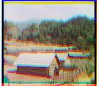
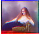
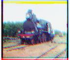
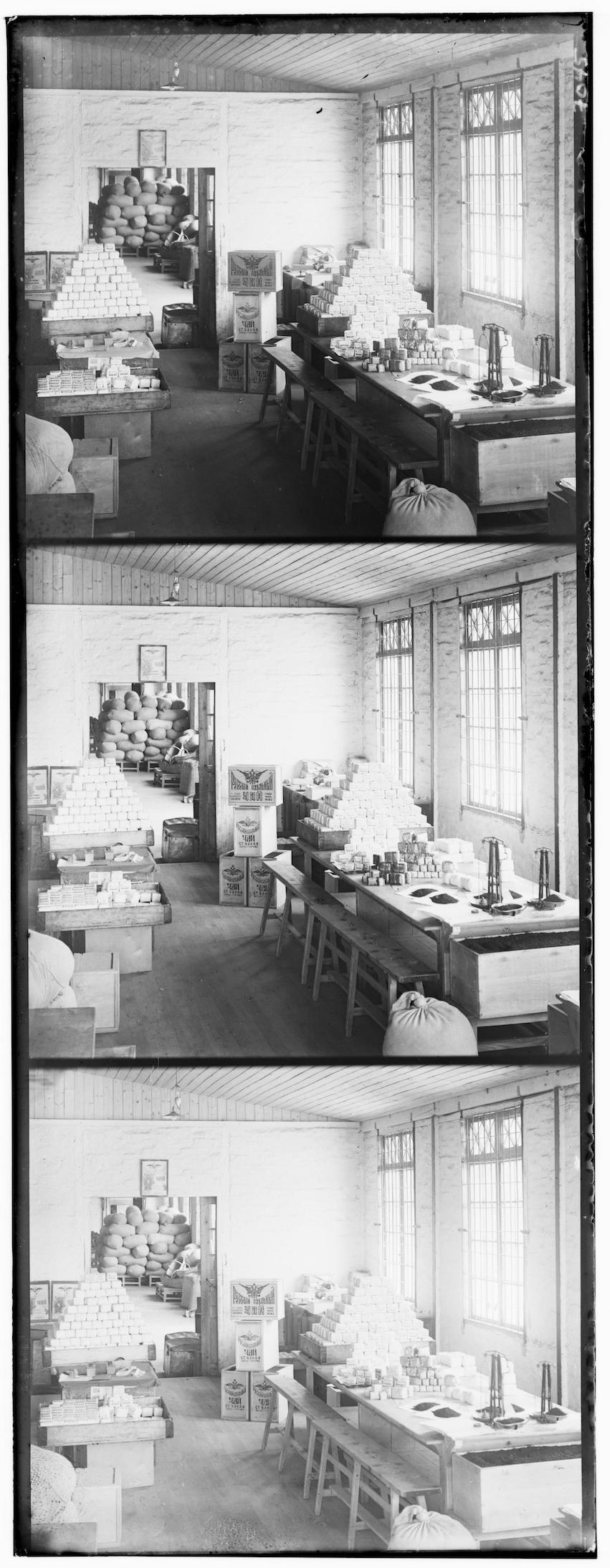
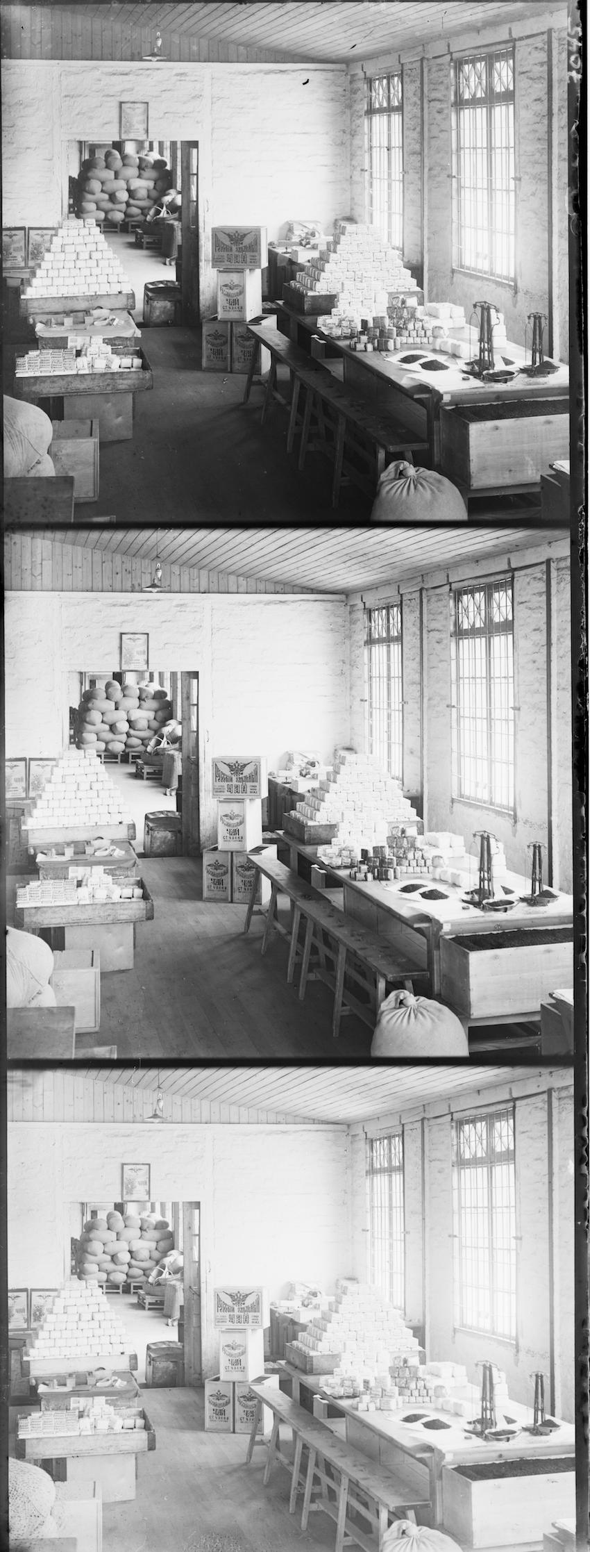
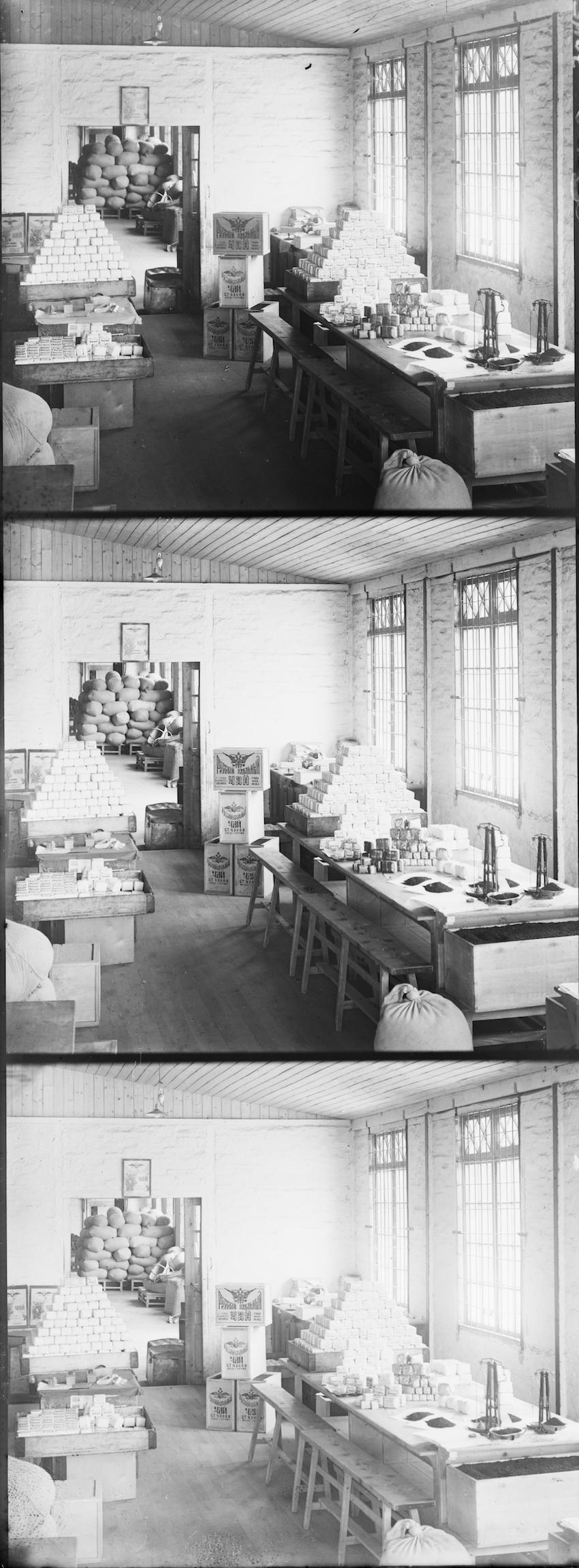
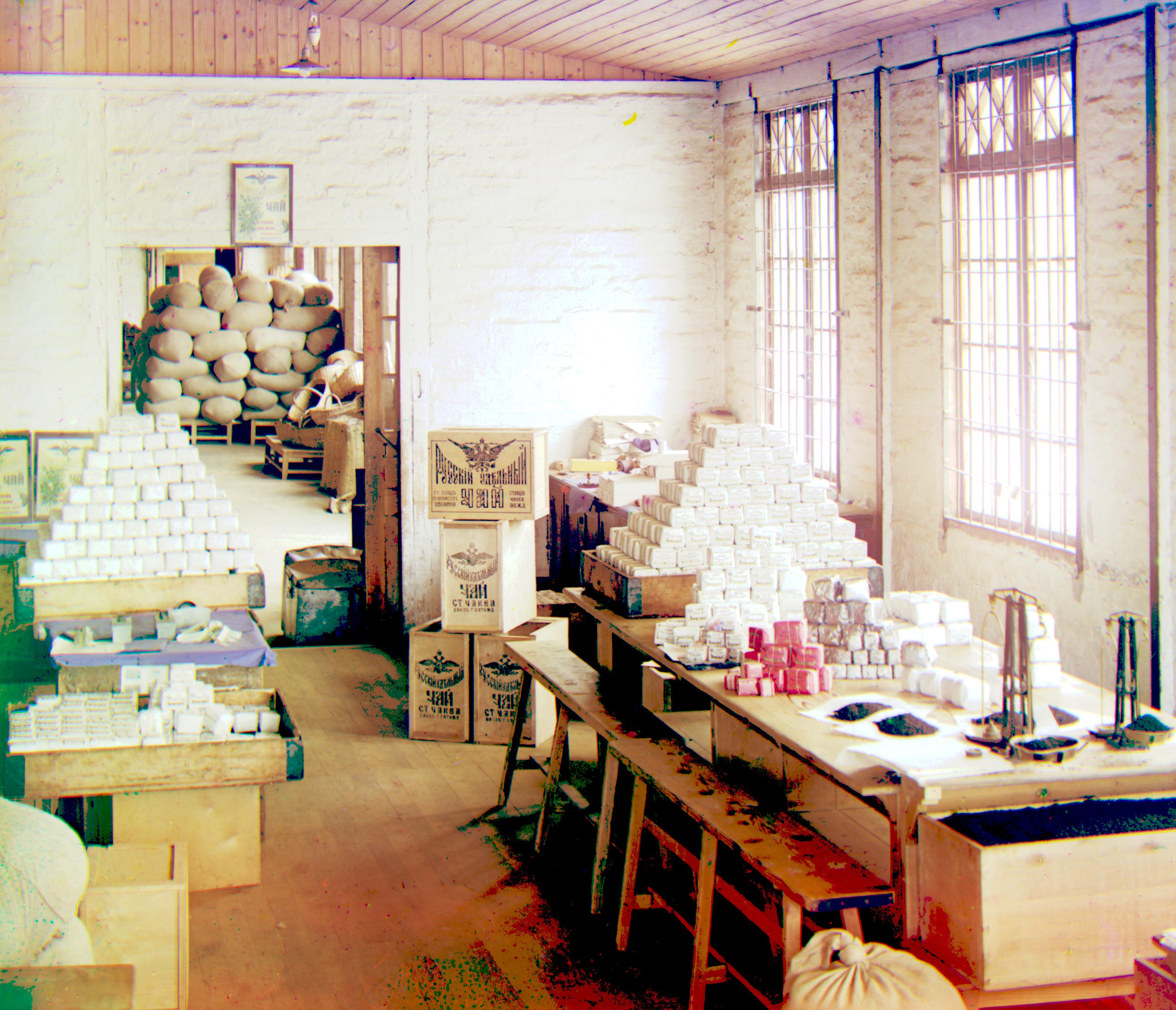
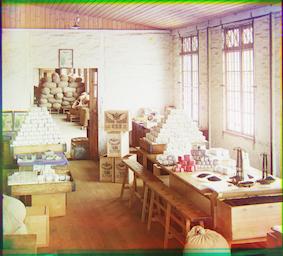
Before we jump into aligning algorithms, let's first convince ourselves why it is necessary to do aligning. Randomly choose three plate file provided and directly stacking them without aligning, we get the images below:
As we can see, this is extremely unsatisfying and painful to appreciate. The main problem here is the color channel of red, blue, and green are placed in improper positions, which resulted in the weird colors and shadows. Therefore, an align process is definitely necessary before stacking channels.
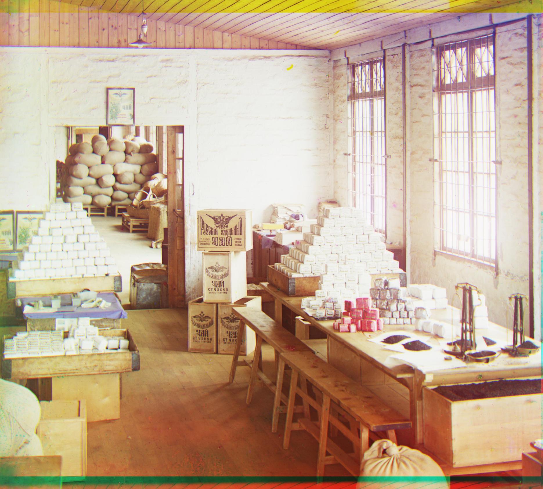
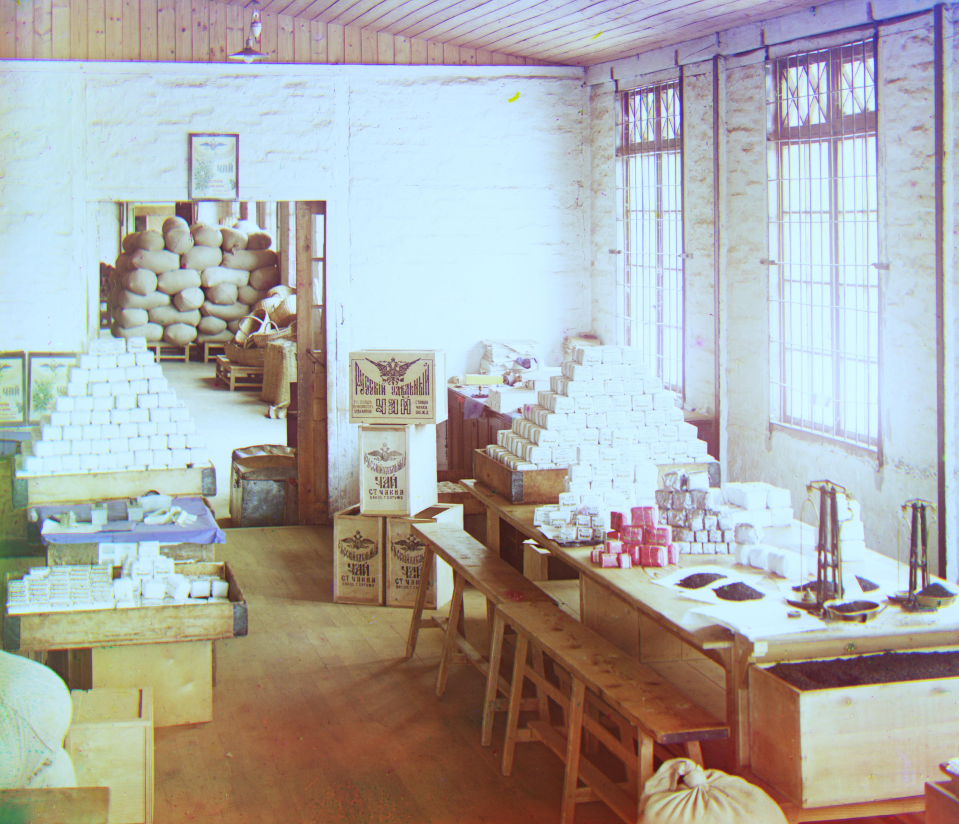
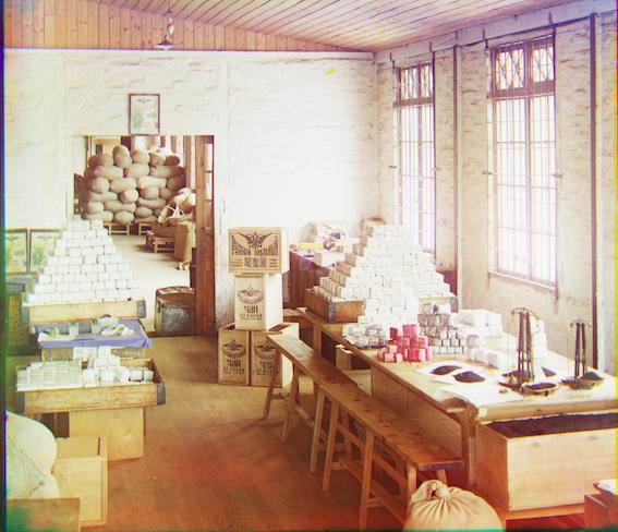
Among the provided digitalized plate images, there are low-resolution JPG files and high-resolution TIF files. We will first examining how to align channels for the smaller pictures. Since the number of pixels along each axis is not exceedingly large, we could try out all possible displacements through iteration and find out which displacement is best through some pre-defined criteria. I utilized a window of (-20, 20) on both x and y axis, and my criteria is to maximize (NCC - SSD) since NCC represent the correlation between the image being aligned and the target, and SDD represents how different they are from each other. As a result, I had the following images:
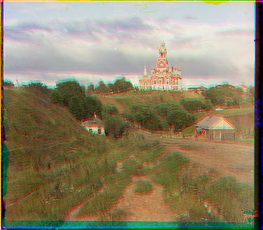
As we can see, the resulting images are much better than the images shown in section 2.0. However, there are indeed room for improvement. For example, the boundaries of the resulting images are abnormal, and pictures themselves can still be improved. We will discuss other improvement techniques later in section 3.
The naive approach introduced above can indeed solve many of the problems, but it will be very time-consuming when an image has great amount of pixels (TIFF files). Therefore, a more efficient algorithm is necessary. Here, I utilized the method of image pyramid to represent the image at multiple scales and update the estimate of best displacement accordingly. In this process, I chose to scale by a factor of 2 and stop when one of the axis has less than 300 pixels. I also increase the size of search window as the pyramid going up (the smaller a image is, the bigger its search window is). Additionally, since TIFF files have more pixels, I made the following two improvements:
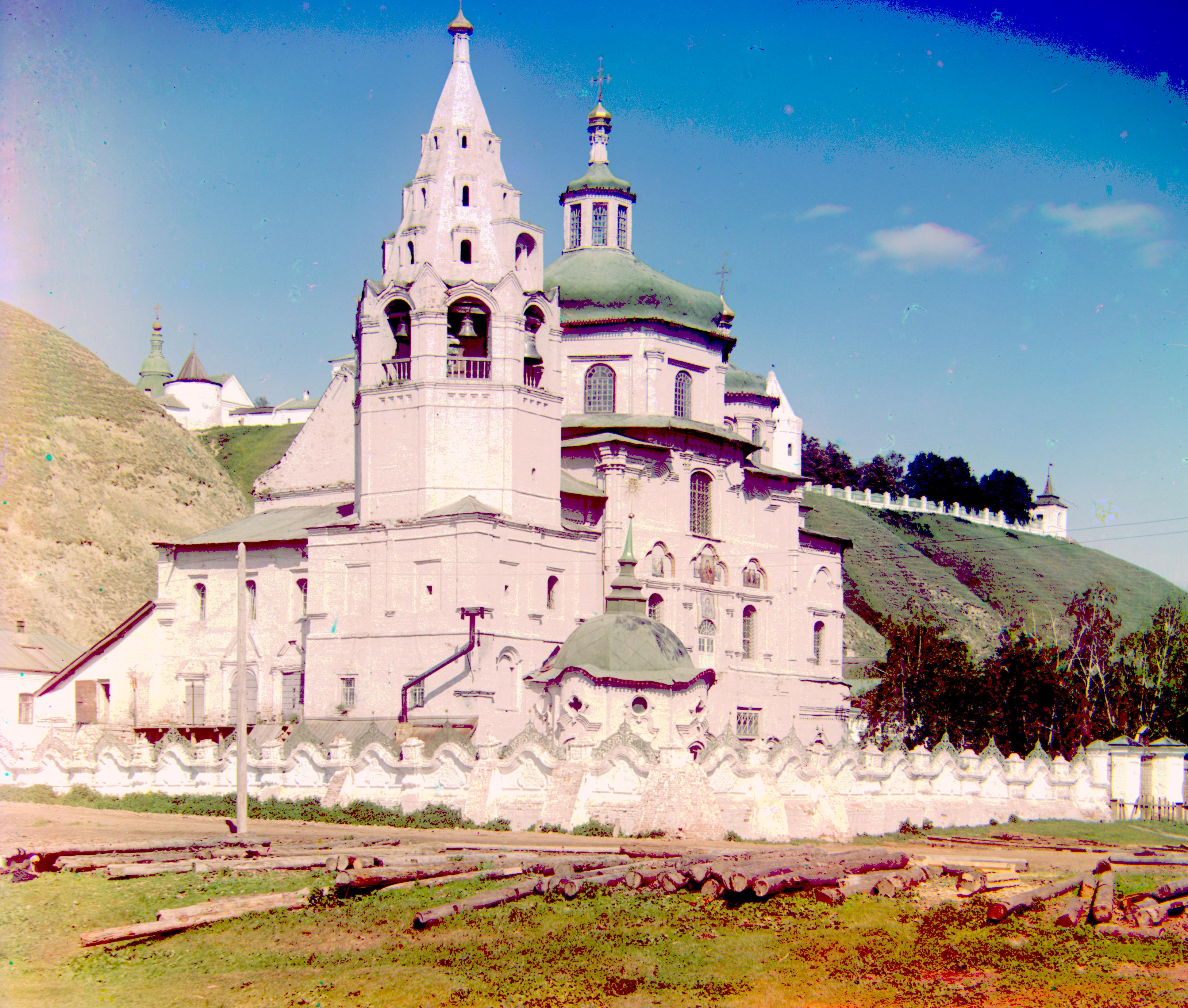
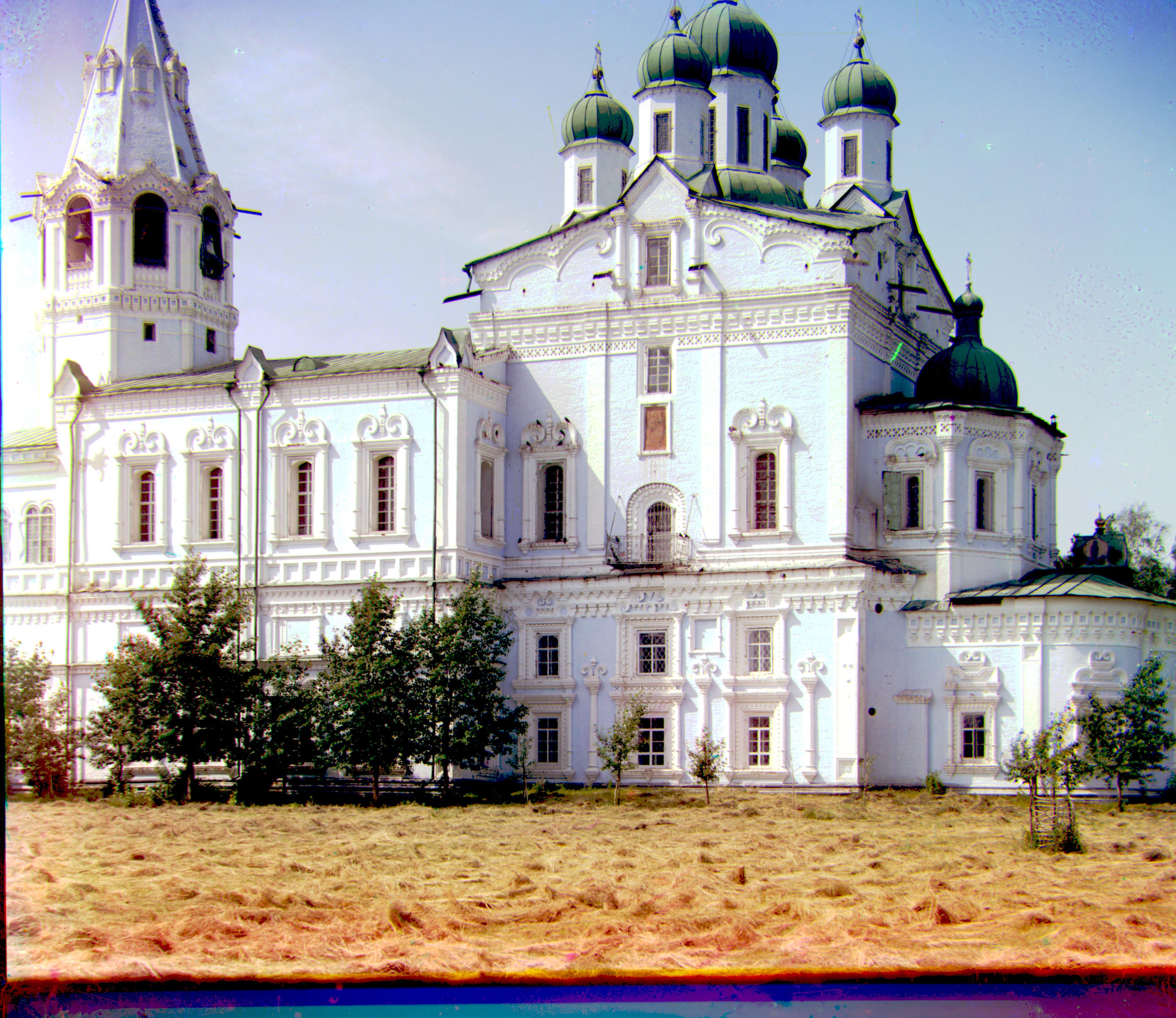
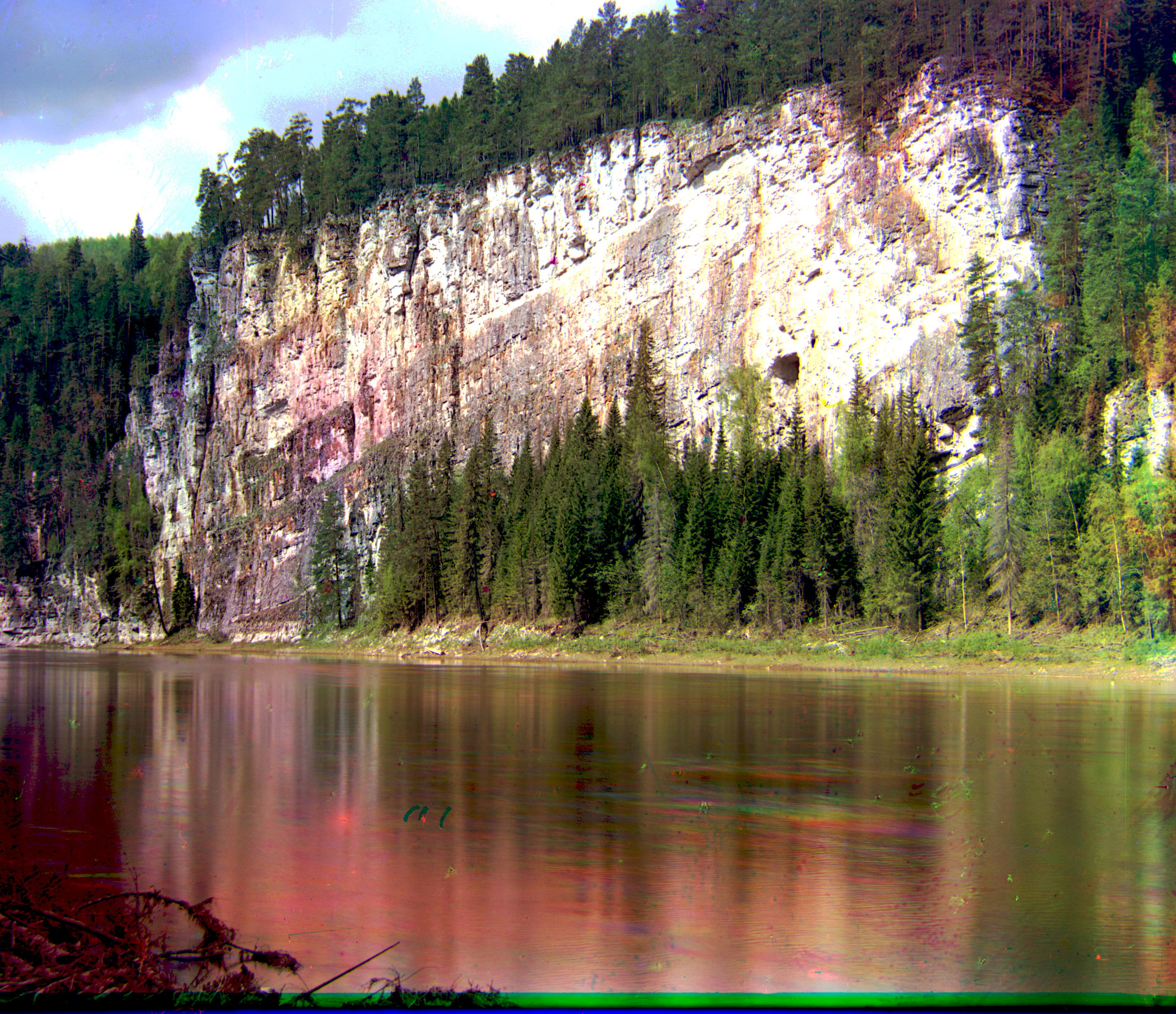
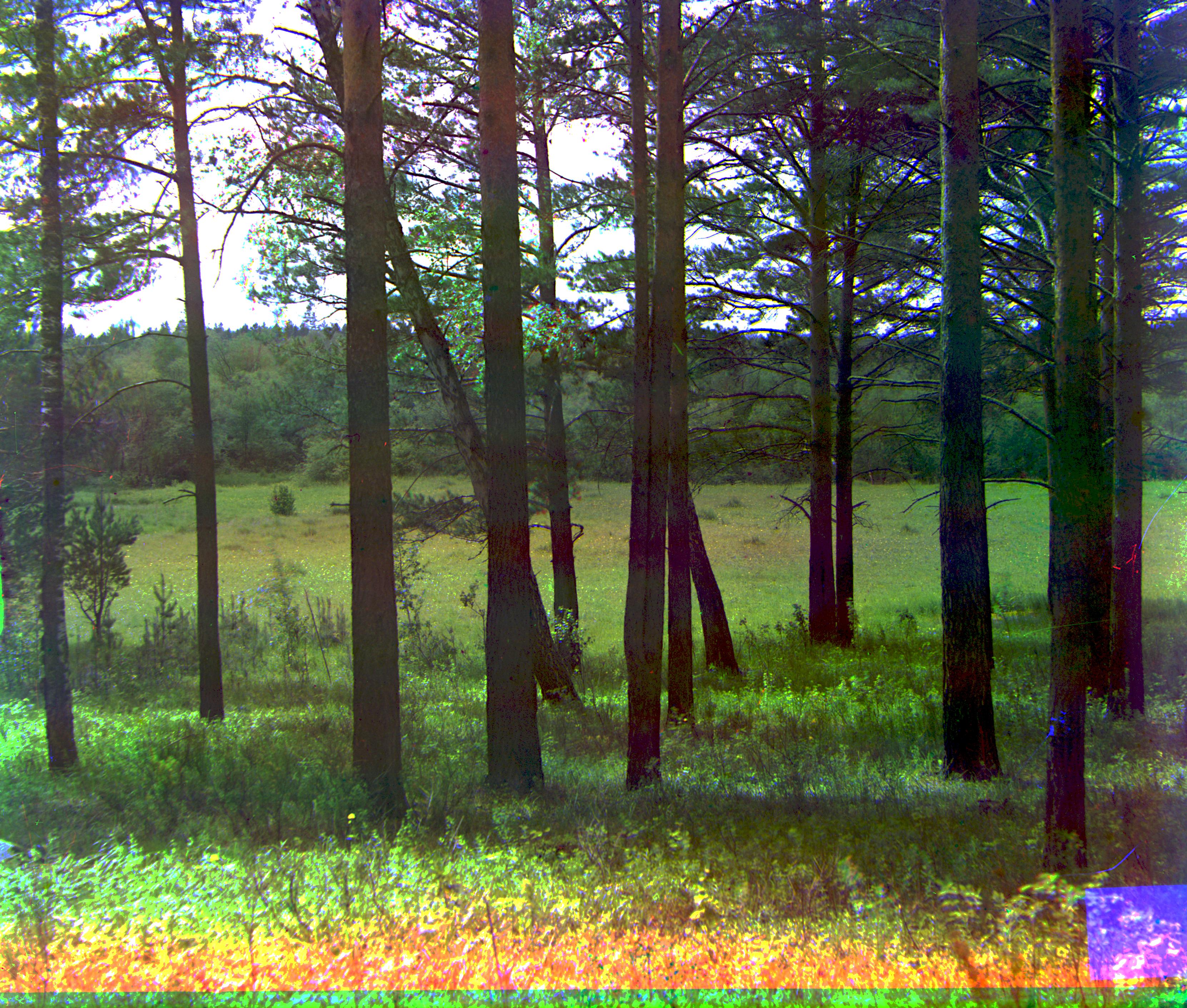
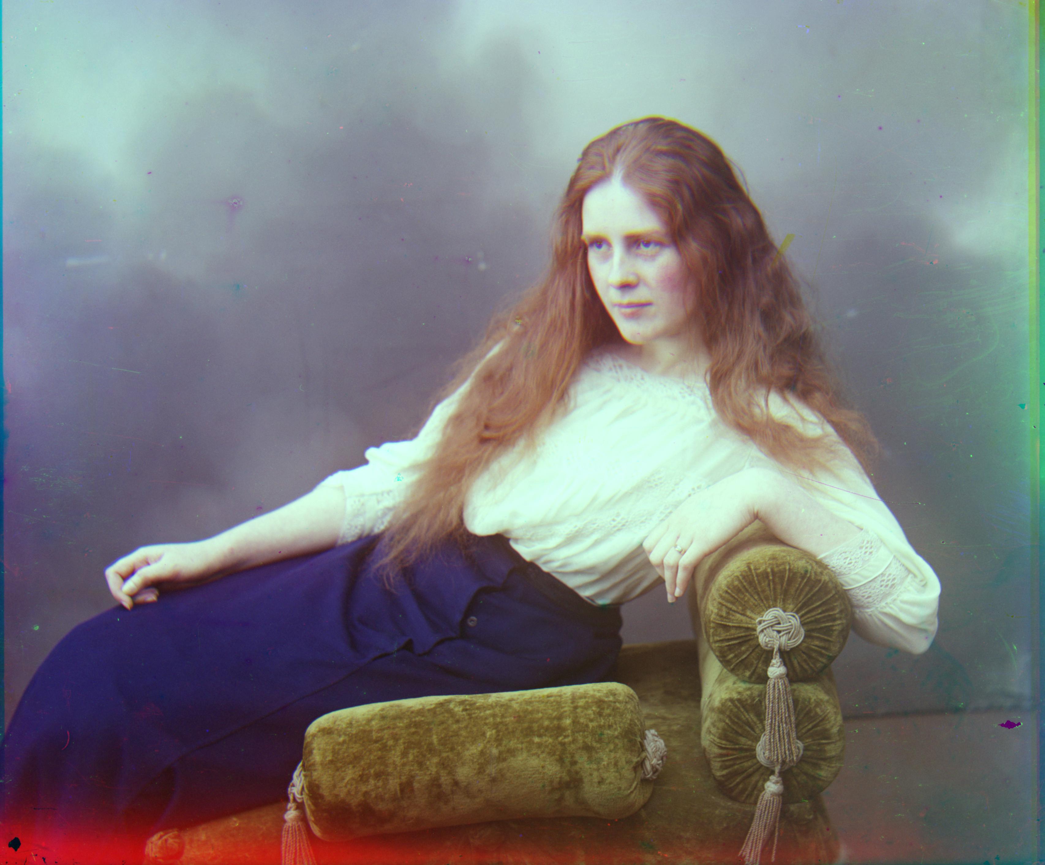
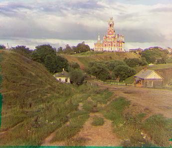
Through the techniques above, I succeeded in aligning the TIFF images and got the resulting pictures as follows. The displacement is shown as < x_shift, y_shift >
In the following sections we will try to do multiple improvements to make our image better.
When looking at the raw pictures, it is not hard to find that the original plate picture has a black & white boundary, which did affect our aligning and picture generation a lot. Before, the approach I took is to crop the image by a fixed ratio. This seems to be better than nothing, but a automatic cropping function is more than handy. For this part, I proposed two algorithms:
The following images show a comparison on how my Bells & Whistles changed the image quality. I only chose a proportion of all output, complete output is uploaded to bCourse:
As we can see from the examples above, the Mask-Cropped did a really good job in cropping the edges, which resulted in a better quality image as well as less black strips in the generated images. However, there is still another problem: the color strips. We will solve this problem in the next section
The colorful strips near the boundary of the images are caused by aligning plates. When we do the displacement, we used np.roll, which will roll back the arrays when out of bound (e.g. the last row will become first row after np.roll(1, axis=1)). Such roll-back schema messed up with our criteria, and will result in weird color strips. In order to solve this problem, I designed another algorithm that after aligning all three plate, the algorithm will detect what's the biggest shift happened, and pad those areas. Thereafter, the cropper we developed above will be able to precisely crop those areas which used to be the color strips. The comparision can be see as follows:
As we can see, the result is very delightening. We managed to get rid of most of the colored edges.
For auto contrasting, I set an threshold for black-like values and white-like values. For all value bigger than WHITE_THRESH, I set the pixel to 1; for all value smaller than BLACK_THRESH, I set the pixel to 0. This approach is naive and I call it autoFixContrast.
As an improvement, I implemented another automatic contrasting algorithm which is more smart. Instead of manually setting a threshold, this algorithm examine the histogram of all three channels. The tail pixels (top and bottom XXX%) are the ones we will change to 0s and 1s. The process is done with histogram distribution of all pixels in one channel, and the corresponding Percent Point Function (PPF) is used to find the tails. I call this autoPropContrast.
Below are the comparisons of the automatic contrasting process. All images are already processed by the algorithms in 3.1 and 3.2:
As we can see, the autoFixContrast does increase the contrast of the image, but its influence tends to vary from picture to picture because the threshold manually set before may not be suitable for all cases. On the other hand, autoPropContract process automatic contrasting proportionally and thus has a much better result. Through comparison, we can see the images produced by autoPropContrast is very colorful and pretty.
The virtual systems of human beings are sensible to colors and are able to capture colors from different object through adjusting the light environment. However, machines such as camera do not have such ability. As a result, the light environment will have significant impact on the photo taken by cameras: the color of a image may be different from its actual color. Therefore, a white balancing algorithm is needed to eliminate the influence of light on color.
Here, I implemented the Gray World Algorithm for processing automatic white balancing function. The essence of the algorithm is that for a colorful image, the average value of R, G, B layer tend to approach to some gray value. Here, I took the average value of all pixels in all layers as the reference gray value. We can then calculate the weight we should apply on each layer based on their individual mean. Finally, by von Kries' color adaption model, we could implement the automatic white balancing procedure.
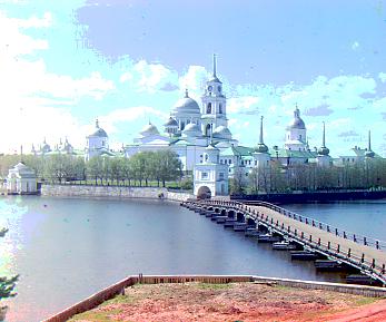
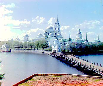
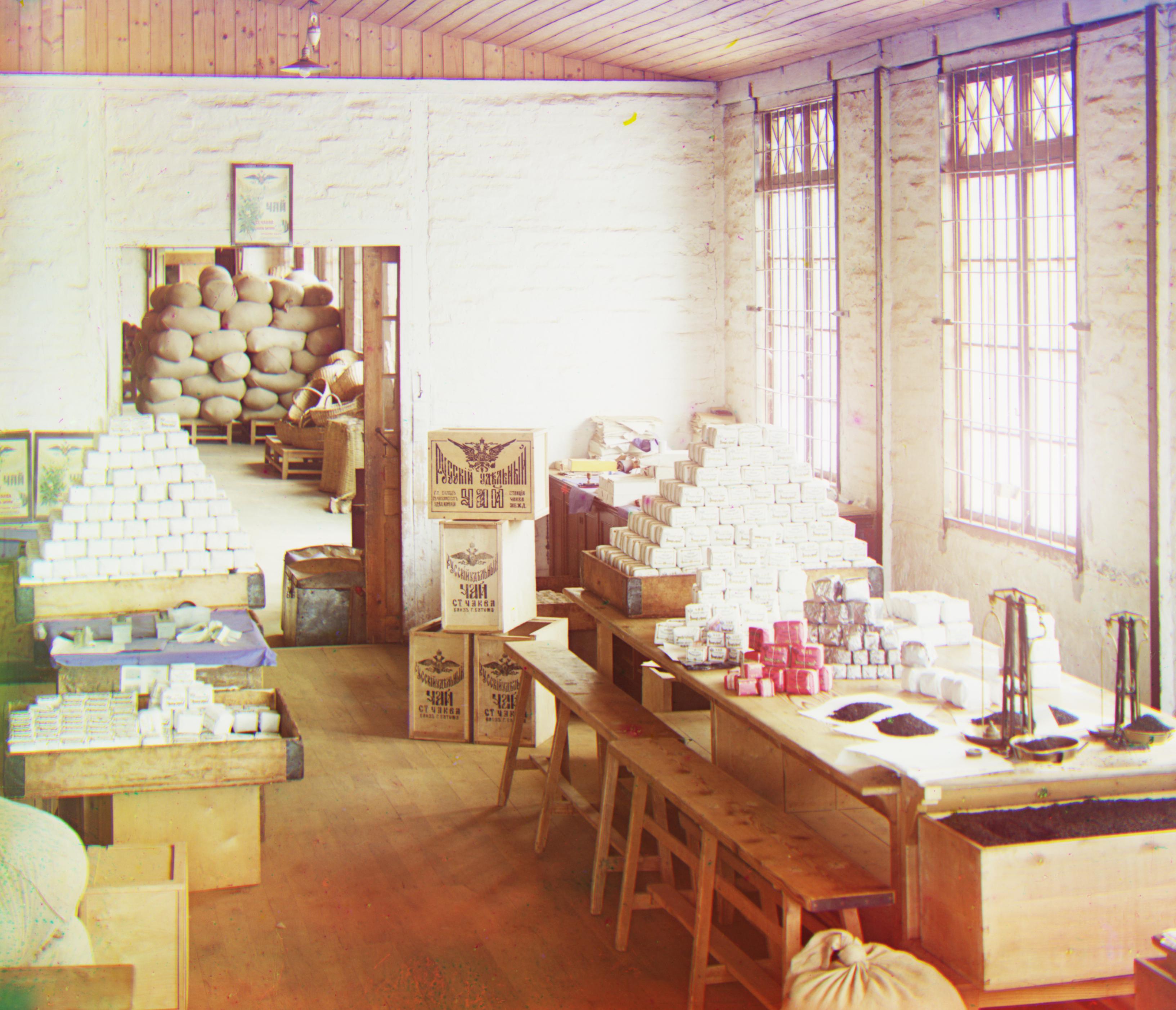
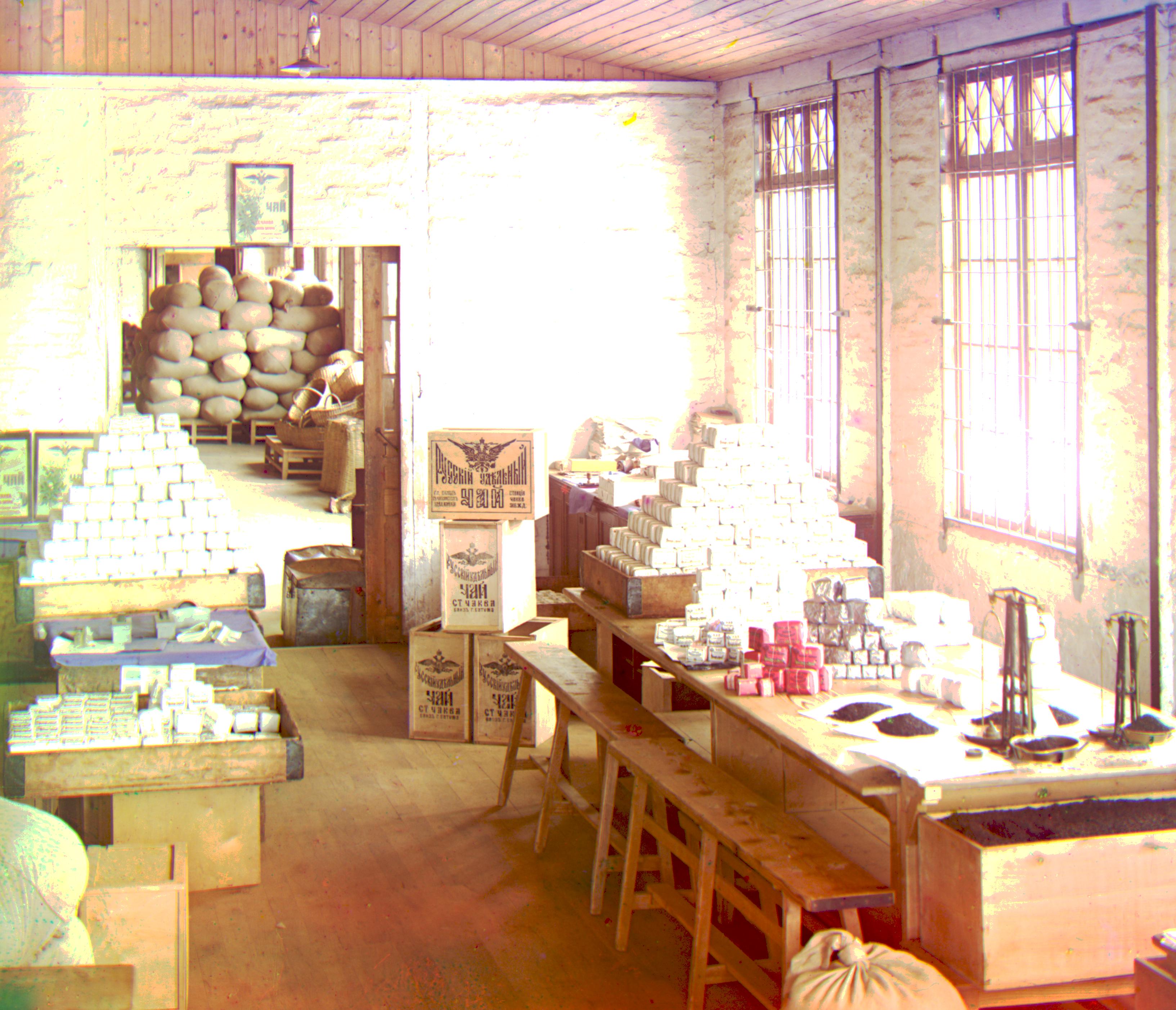
The images below are the images before and after applying white balancing. We can see the obvious difference in color for images before and after white balancing.
For all pictures above, we directly used the R, G, B for shifting and calculating the correlation scores. However, since the brightness in all three layers may be far different from each other, directly comparing the pixels seems unreasonable. Therefore, in this section, I used the sobel filter from skimage module, which will detect the edges in a picture. Thereafter, I will use the filtered image for obtaining align displacement. A comparison is shown as follows. You will need to make the screen brighter in order to see the lines in sobel pictures.
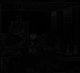 green
green
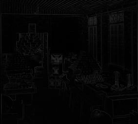 blue
blue
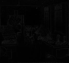
As we can see, using sobel filter did make some difference in the image generated. This technique will be significantly important and helpful when the edge in picture are obvious and the light condition in three layers differs a lot.
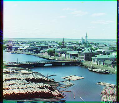
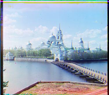
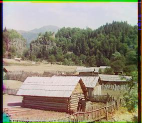
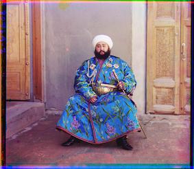
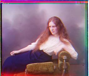
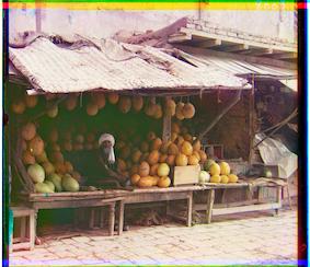
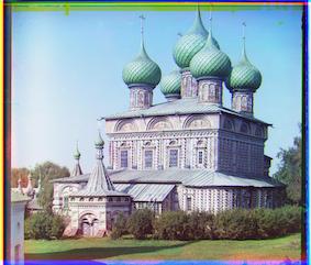
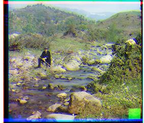
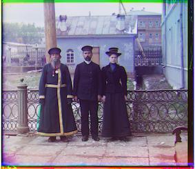
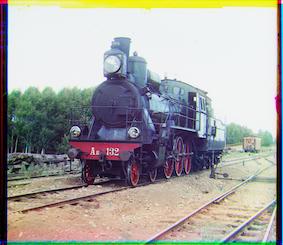
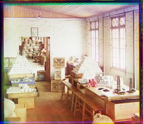
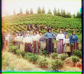
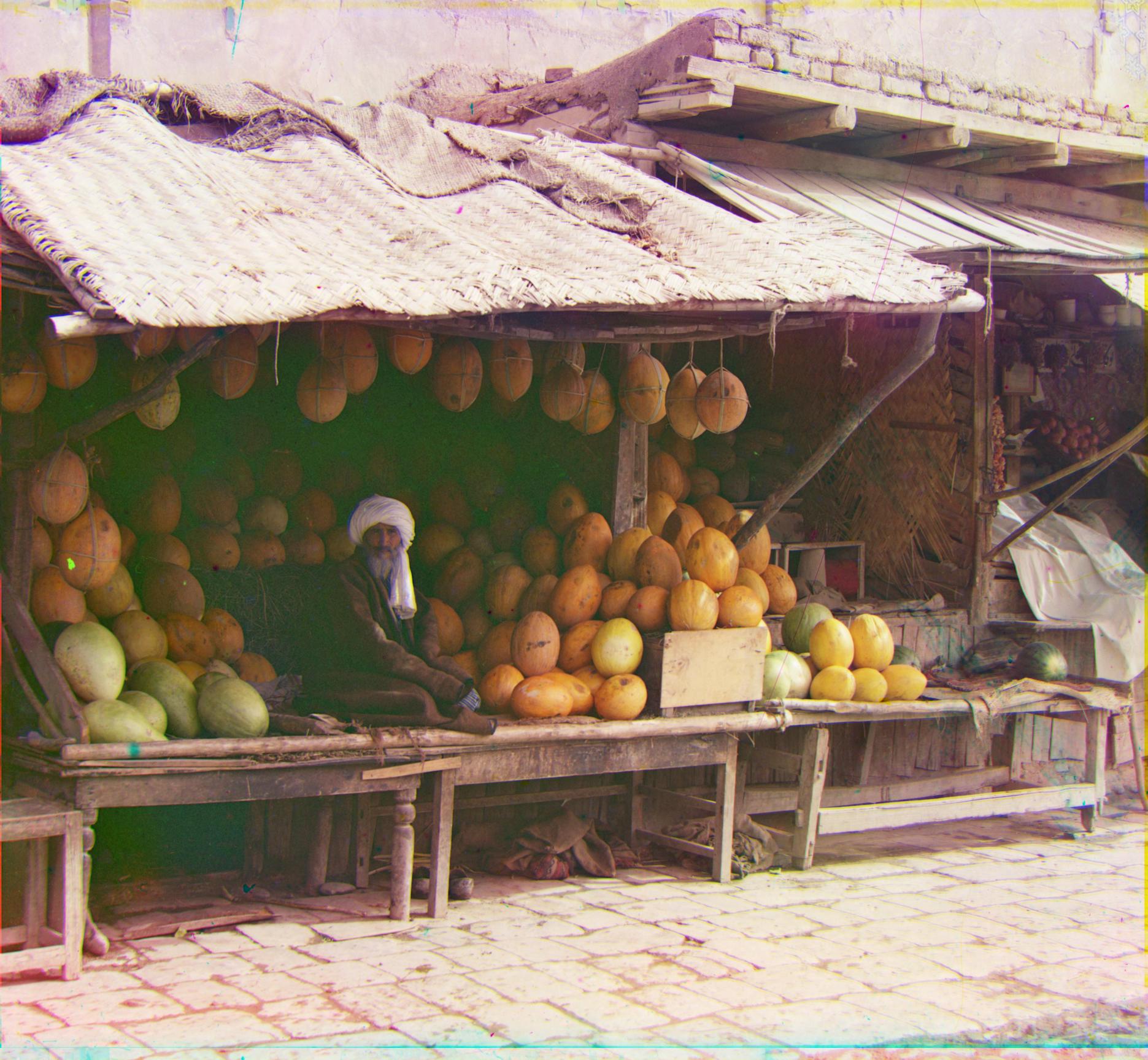
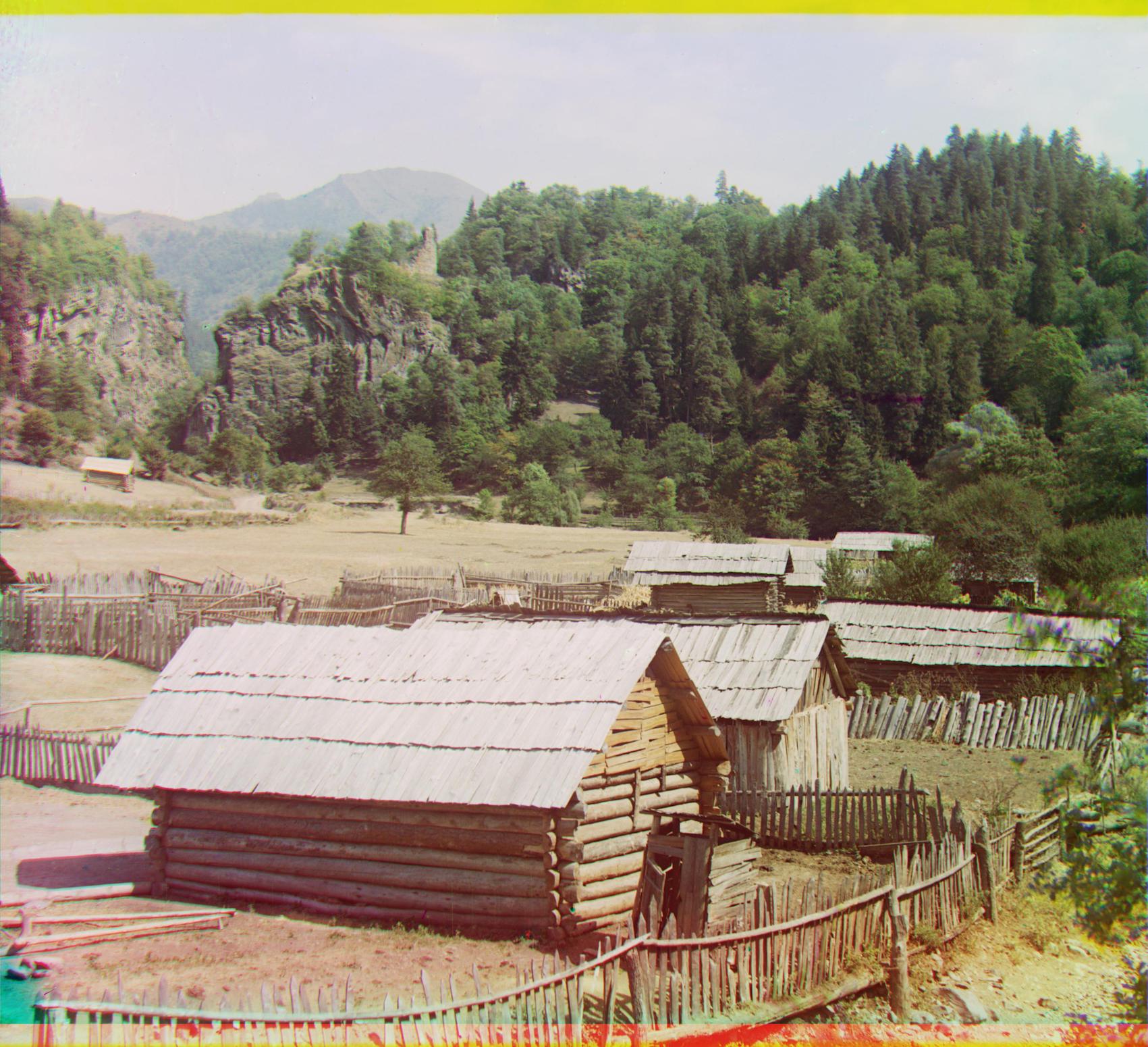
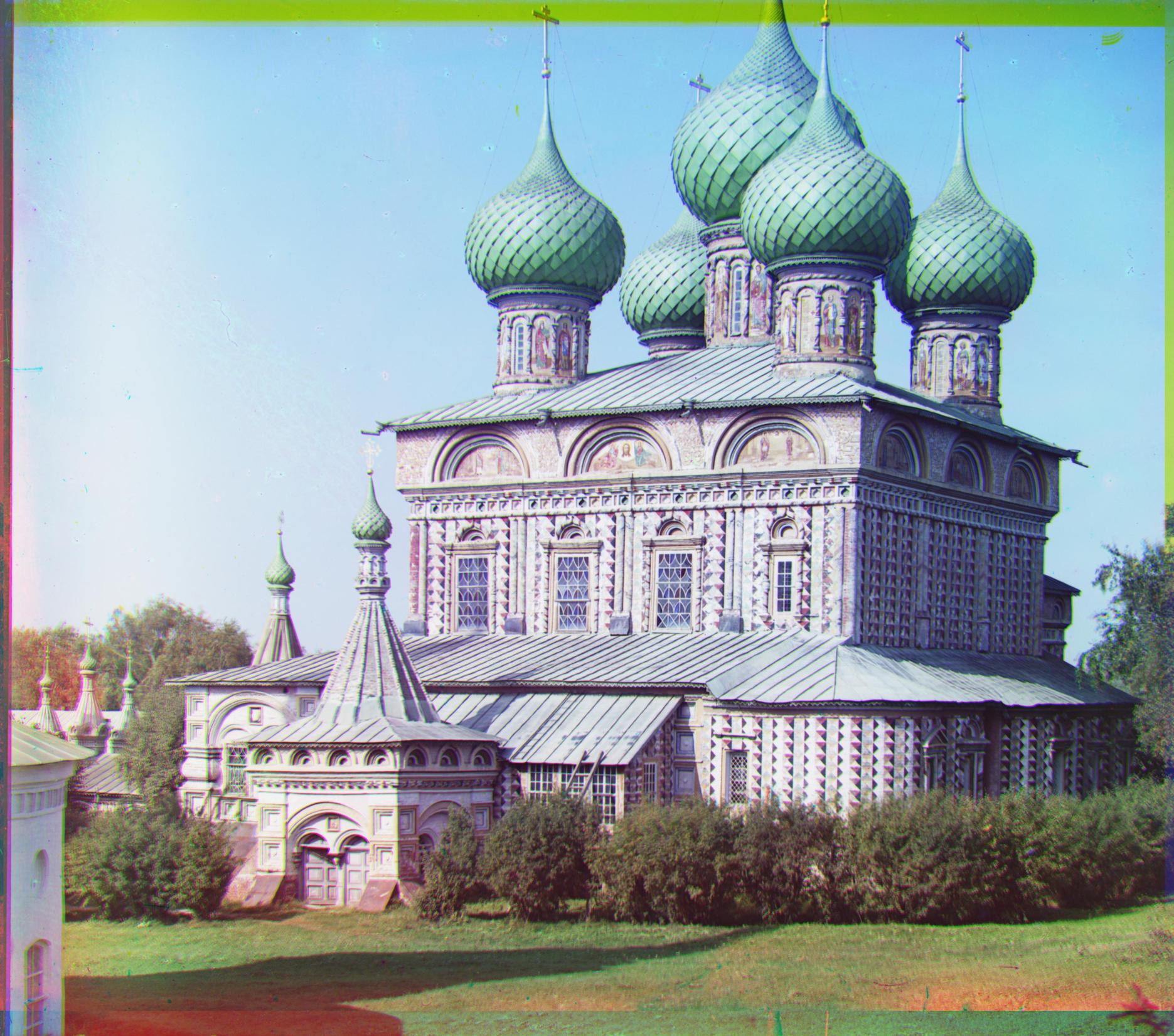
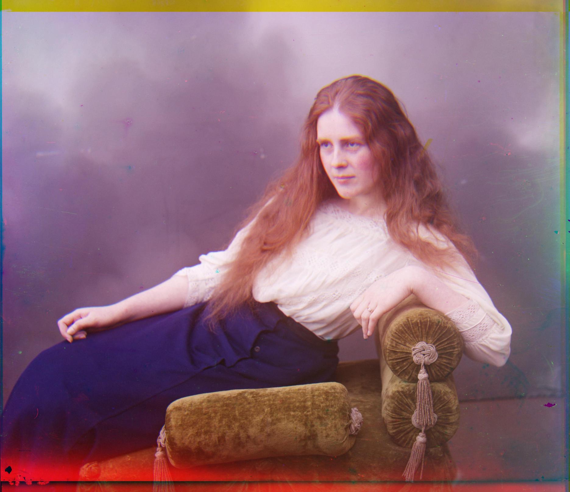
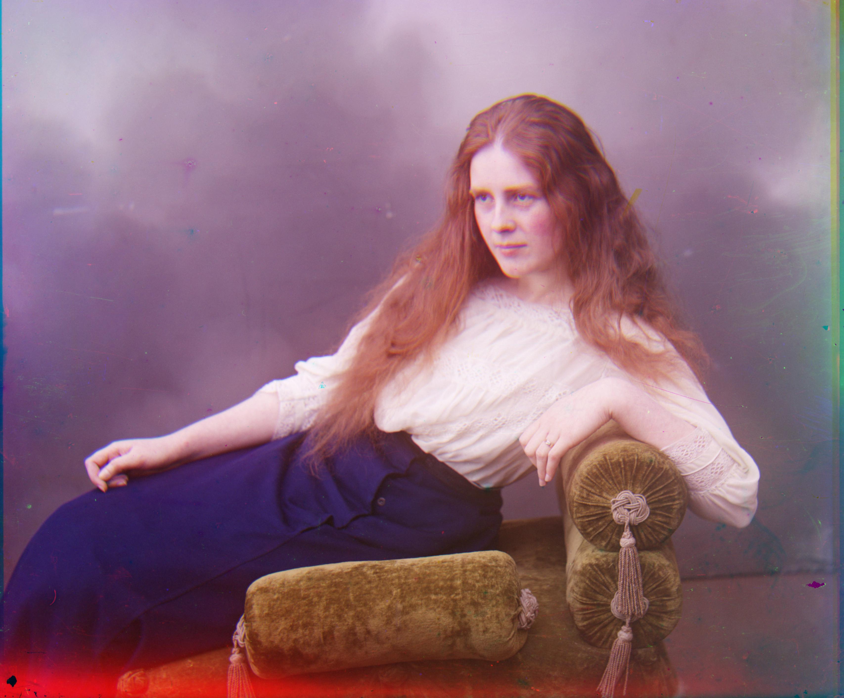
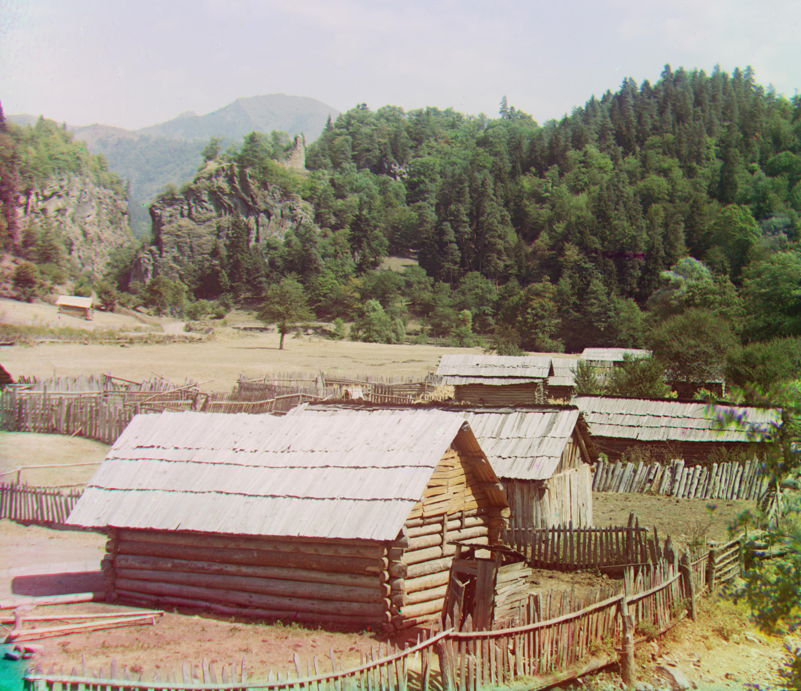
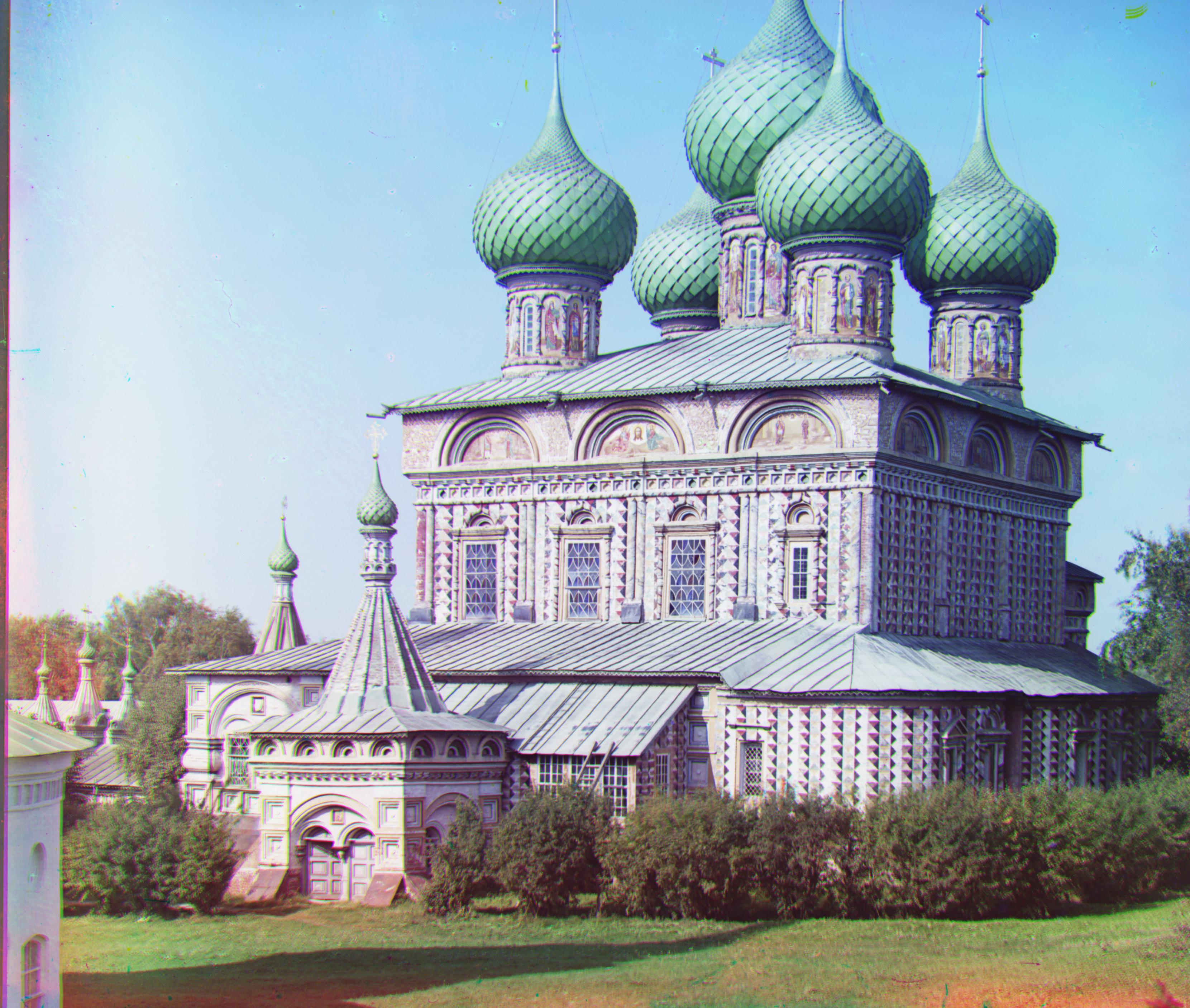
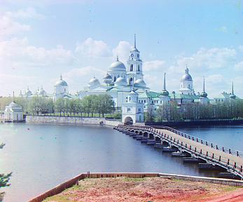
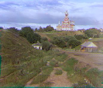
The following pictures are generated through all techniques mentioned above.