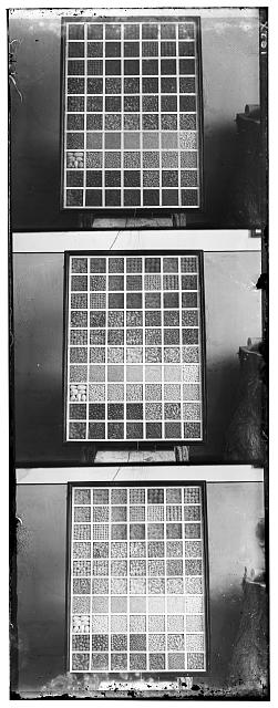
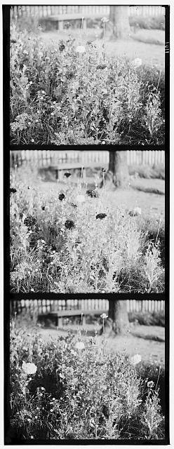
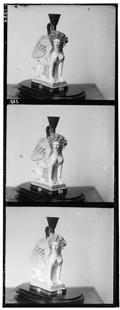
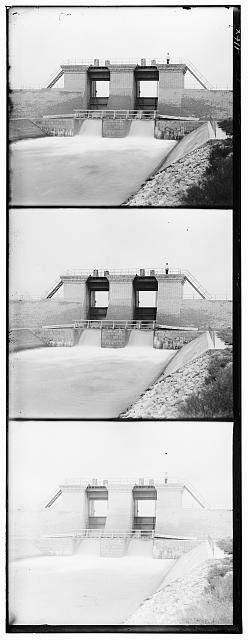
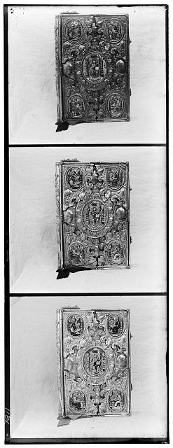
(-1,1).jpg)
— R(1,-8) G(1,-1) |
(6,0).jpg)
— R(-1,-10) G(0,6) |
(-3,-2).jpg)
— R(-3,-7) G(-2,-3) |
To align the three color channels, I implemented both the sum of squared differences (SSD), and the normalized cross-correlation (NCC) algorithms. As a general rule, the NCC performed better from a quality perspective, and had a negligible time tradeoff. The search offset I used was 15 pixels. It must also be mentioned that using np.roll() instead of for-loops had a tremendous impact on performance, providing over 200% speedup on channel alignment – from over 20 seconds needed to reconstruct an image to less than 1. Cheers to the friends who implemented those CPU vectors!
The figures below and in the next sections are accompanied by the shifts of their color channels, according to the key: color_channel(horizontal shift, vertical shift).
|
— R(1,-8) G(1,-1) |
— R(-1,-10) G(0,6) |
— R(-3,-7) G(-2,-3) |
To speed up the runtime for large inputs, I also implemented image pyramids. Namely, using a user-specified L (levels) and α (pyramid factor) variables, I iteratively (yes, iteratively, not recursively... !) construct a pyramid by rescaling a given channel by α until L is reached. The data structure I employed for the pyramid is a deque from the default collection, due to its simplicity in comparison to a list – after all, the pyramid only needs to support prepending.
Furthermore, it is worth noting that I rescale the channels at each level without antialiasing them, because after having experimented with both options, I could observe no practical difference. Antialiasing costs Ω(L) time that can simply be saved. I originally expected antialiasing to improve the quality of the output image, but I now hypothesize that upon advancing to the next pyramid level, any small error from rescaling alias is easily corrected, because it is within the search offset.
Overall, pyramids significantly improved speedup, with all images requiring less than 8 seconds to align using the default parameters. For timing tests, I used Python's time library. Of course, even though all images were aligned quickly, not all were also aligned correctly. It was about time to implement a few Bells & Whistles...
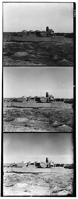
(-43,-3).jpg)
— R(-2-110) G(-3,-43) |
(2,-2).jpg)
— R(-18,-114) G(-2,2) |
(-141,-1).jpg)
— R(-2,-141) G(-1,-141) |
(-43,-14).jpg)
— R(-21,-107) G(-14,-43) |
(-58,2).jpg)
— R(4,-141) G(2,-58) |
(-91,-1).jpg)
— R(-2,-198) G(-1,-91) |
(-64,-21).jpg)
— R(-36,-129) G(-21,-64) |
(-55,1).jpg)
— R(1,-143) G(1,-55) |
(-64,-3).jpg)
— R(-2,-129) G(-3,-64) |
(-131,2).jpg)
— R(-1,-114) G(2,-131) |
(-167,2).jpg)
— R(3,-134) G(2,-167) |
(-64,-1).jpg)
— R(4,-76) G(-1,-64) |
Although pyramids guarantee that even the largest of images will be relatively well aligned in a reasonable amount of time, such alignment is far from perfect. If anything, the Monastery, the Emir, the Harvesters, the Village and the Workshop images are badly aligned, and so in a striking manner. To achieve better results I hence had to devise certain strategies, out of which four proved effective.
The first strategy was to simply increase the pyramid factor α, at the cost of time. Higher α means that the images stored in the pyramid will be larger, and therefore a larger number of pixels will be available to test for alignment. The more α approaches 1, the smaller the pyramid speedup. In practice, I found that 0.85 is a good compromise between quality and speed, with even the largest of images requiring less than 8 seconds to process when using 16-level pyramids.
The second strategy was to crop the images before performing any alignment tests, to remove noise present around borders. This drastically improved the output image, with its effects being most noticeable in smaller images, especially the Monastery.
(-8,-1).jpg)
— 10% Crop |
— Original Size |
(-7,-1).jpg)
— 10% Crop |
— Original Size |
(-5,-1).jpg)
— 10% Crop |
— Original Size |
The third, and somewhat controversial strategy, was to align images based on the green, rather than the blue channel. In theory, using any channel as a base should yield similar results, unless the filter used to construct it is deffective. Perhaps Prokudin-Gorskii's green filter was at a better condition than his blue filter. Or perhaps, because photography took place under sunlight, the majority of which is green light, images passed by the green filter were graphed using more light. It appears more reasonable to alignt two low-exposure images with a high-exposure image, rather than a low-exposure and a high-exposure image with a low-exposure image. However, the above are merely hypotheses: I could not find any reliable sources on the topic. Yet for all practical purposes, aligning based on the green channel yielded better results; notice the stark difference between the green-based and blue-based versions of the Harvesters, and the cropped Emir.
(-76,1).jpg)
— Green Base, Original Size |
— Blue Base, Original Size |
(-64,-18).jpg)
— Green Base, 10% Crop |
(-55,-21).jpg)
— Blue Base, 10% Crop |
The fourth, and final strategy, was to perform edge detection on the channels before attempting to align them. Since all three channels are low contrast images (the range of their shades is limited) and contain noise, pixels representing clearly distinct parts of the desired image may have relatively similar shades, which skews the metric. The solution is to ensure that any difference in color also encodes for a difference in characteristics, and that such difference is sharp. This can be achieved through edge detectors: filters that enhance the edges (the parts of an image giving rise to its characteristics) and that dim everything else. After experimenting with a number of them, including Sobel, SUSAN, and few hessian-based ones, the ones that stood out were Canny and Sato. Although Sato is primarily aimed at biomedical uses (to detect "tubeness") it works surprisingly well for the given set of images. The following figures compare Sato with Canny. The latter is marginally more effective.
(-67,-1).jpg)
— Sato — B(2,28) R(-1,-67) |
(-67,1).jpg)
— Canny — B(2,31) R(1,-67) |
(-58,-7).jpg)
— Sato — B(20,50) R(-7,-58) |
(-58,-7).jpg)
— Canny — B(22,50) R(-7,-58) |
(-67,2).jpg)
— Sato — B(8,64) R(2,-67) |
(-67,2).jpg)
— Canny — B(7,64) R(2,-67) |
(-45,-3).jpg)
— Sato — B(8,41) R(-3,-45) |
(-45,-3).jpg)
— Canny — B(7,41) R(-3,-45) |
(-64,-2).jpg)
— Sato — B(4,55) R(-2,-64) |
(-64,-2).jpg)
— Canny — B(4,58) R(-2,-64) |
(-102,-2).jpg)
— Sato — B(5,86) R(-2,-102) |
(-101,-2).jpg)
— Canny — B(6,86) R(-2,-101) |
(-55,-5).jpg)
— Sato — B(20,53) R(-5,-55) |
(-55,-5).jpg)
— Canny — B(18,53) R(-5,-55) |
(-104,-4).jpg)
— Sato — B(26,82) R(-4,-104) |
(-104,-4).jpg)
— Canny — B(26,82) R(-4,-104) |
(-61,0).jpg)
— Sato — B(6,55) R(0,-61) |
(-61,3).jpg)
— Canny — B(7,58) R(3,-61) |
(-44,-24).jpg)
— Sato — B(3,44) R(-24,-44) |
(-44,-24).jpg)
— Canny — B(1,41) R(-24,-44) |
(-75,-5).jpg)
— Sato — B(5,67) R(-5,-75) |
(-75,-5).jpg)
— Canny — B(5,67) R(-5,-75) |
(-53,5).jpg)
— Sato — B(1,53) R(5,-53) |
(-53,5).jpg)
— Canny — B(0,53) R(5,-53) |
As a final touch, the images may be post-processed to appear more photorealistic. By default, they are low contrast (dark spots are not very dark, and bright spots are not very bright) and are overexposed (light sources emit too much light). The most popular technique to address such problem is histogram equalization (that is, spreading the tones of each color channel over all discrete values between 0 and 1). However, after playing around with some of my own functions and skimage methods, I discovered that histogram equalization made the images look even more exposed and unnatural; it "overcompensated" for the problem.
The solution I eventually found is called sigmoid contrast adjustment. Namely, by transforming the image using a sigmoid function, rather than, say, the cumulative distribution, it becomes possible to auto-contrast the image and still preserve somewhat natural-looking light. Implementation-wise, I used the adjust_sigmoid() from skimage.exposure, with a cuttoff of 0.5, and gain of 6 (where any gain above 5 increases contrast, and anything below reduces it). The figures below demonstrate sigmoid adjustment in action. Notice how images on the left, where the sigmoid has been applied look natural, yet more vivid than the untouched images on the right.
(-67,1).jpg)
— Sigmoid |
— Untouched |
(-58,-7).jpg)
— Sigmoid |
— Untouched |
(-67,2).jpg)
— Sigmoid |
— Untouched |
(-45,-3).jpg)
— Sigmoid |
— Untouched |
(-64,-2).jpg)
— Sigmoid |
— Untouched |
(-101,-2).jpg)
— Sigmoid |
— Untouched |
(-55,-5).jpg)
— Sigmoid |
— Untouched |
(-104,-4).jpg)
— Sigmoid |
— Untouched |
(-61,3).jpg)
— Sigmoid |
— Untouched |
(-44,-24).jpg)
— Sigmoid |
— Untouched |
(-75,-5).jpg)
— Sigmoid |
— Untouched |
(-53,5).jpg)
— Sigmoid |
— Untouched |
|
|
|
(-68,41).jpg)
— B(-37,44) R(41,-68) |
||
(-53,-3).jpg)
— B(4,3) R(-3,-53) |
||
(-94,-20).jpg)
— B(22,18) R(-20,-94) |
|
|
|
(-61,-6).jpg)
— B(7,50) R(-6,-61) |
(-45,6).jpg)
— B(-6,37) R(6,-45) |
(-48,0).jpg)
— B(1,26) R(0,-48) |