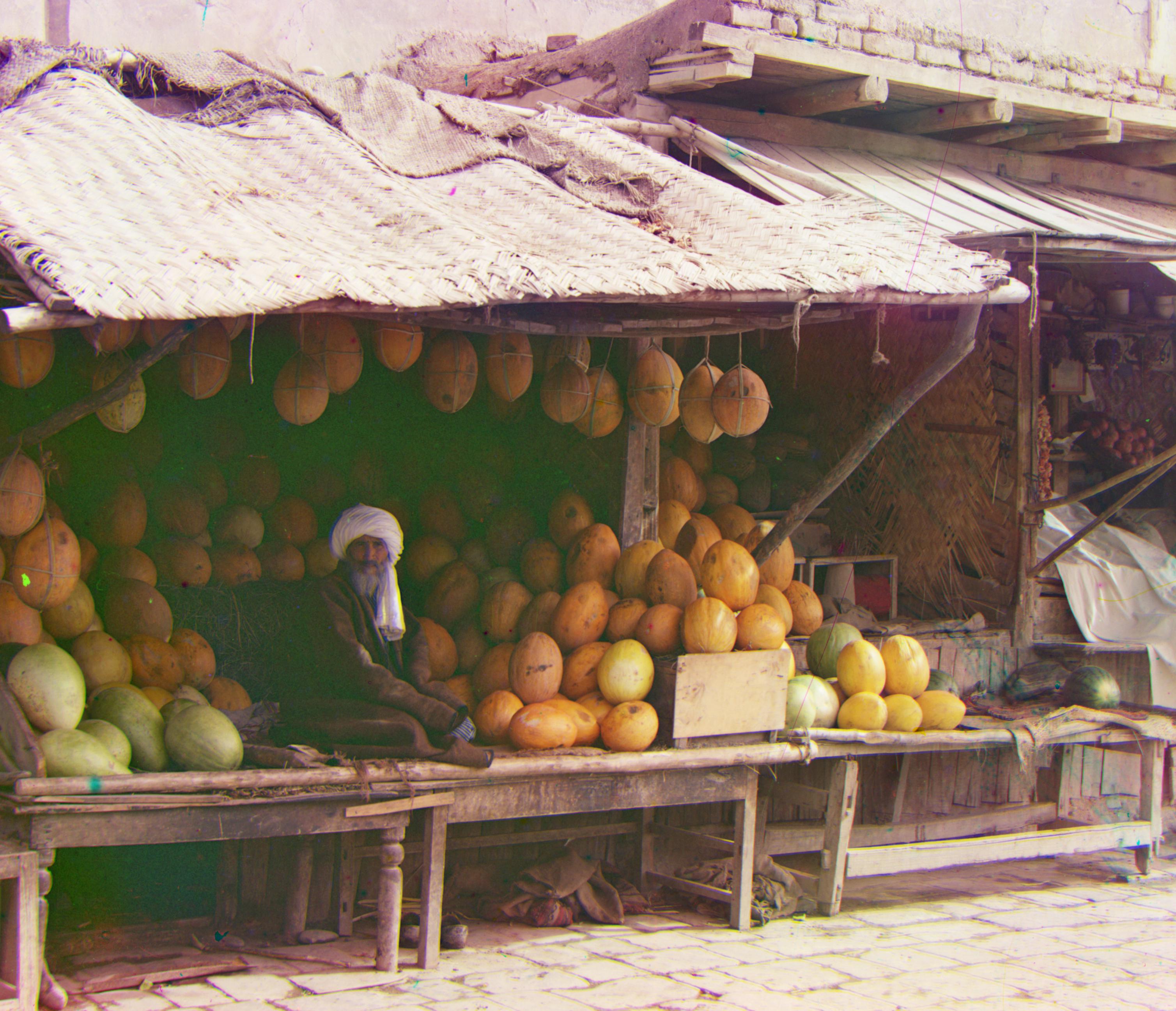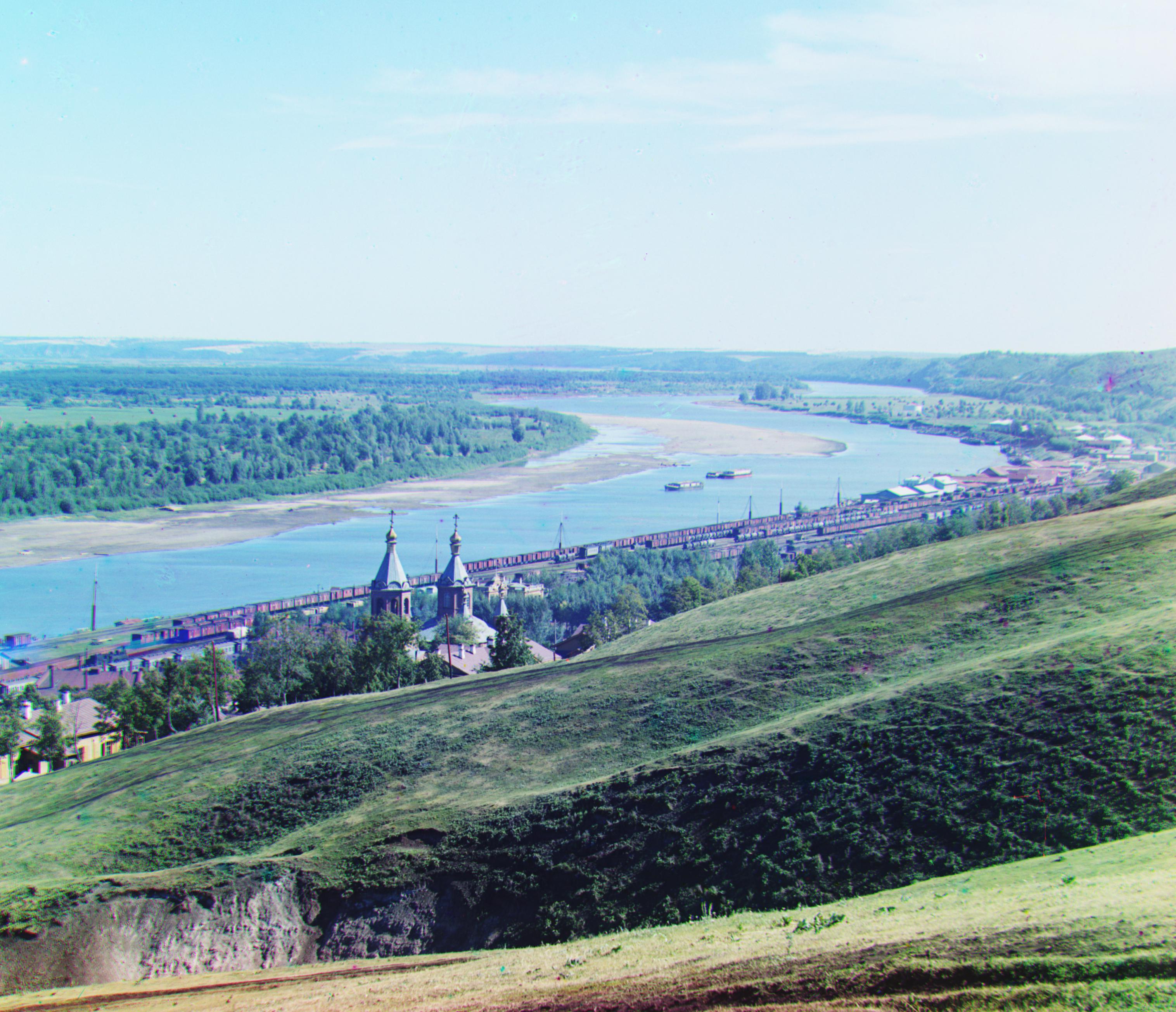


In the 20th century, a photographer named Sergei Mikhailovich Prokudin-Gorskii had an idea. He believed that color photography could be achieved if you record three exposures of every scene onto a glass plate using a red, a green, and a blue filter. He used a three-stack camera, with a different colored glass plate on each lense. Unfortunately, he wasn't able to see his project through. However, his RGB glass plate negatives have been digitized and made them available online.
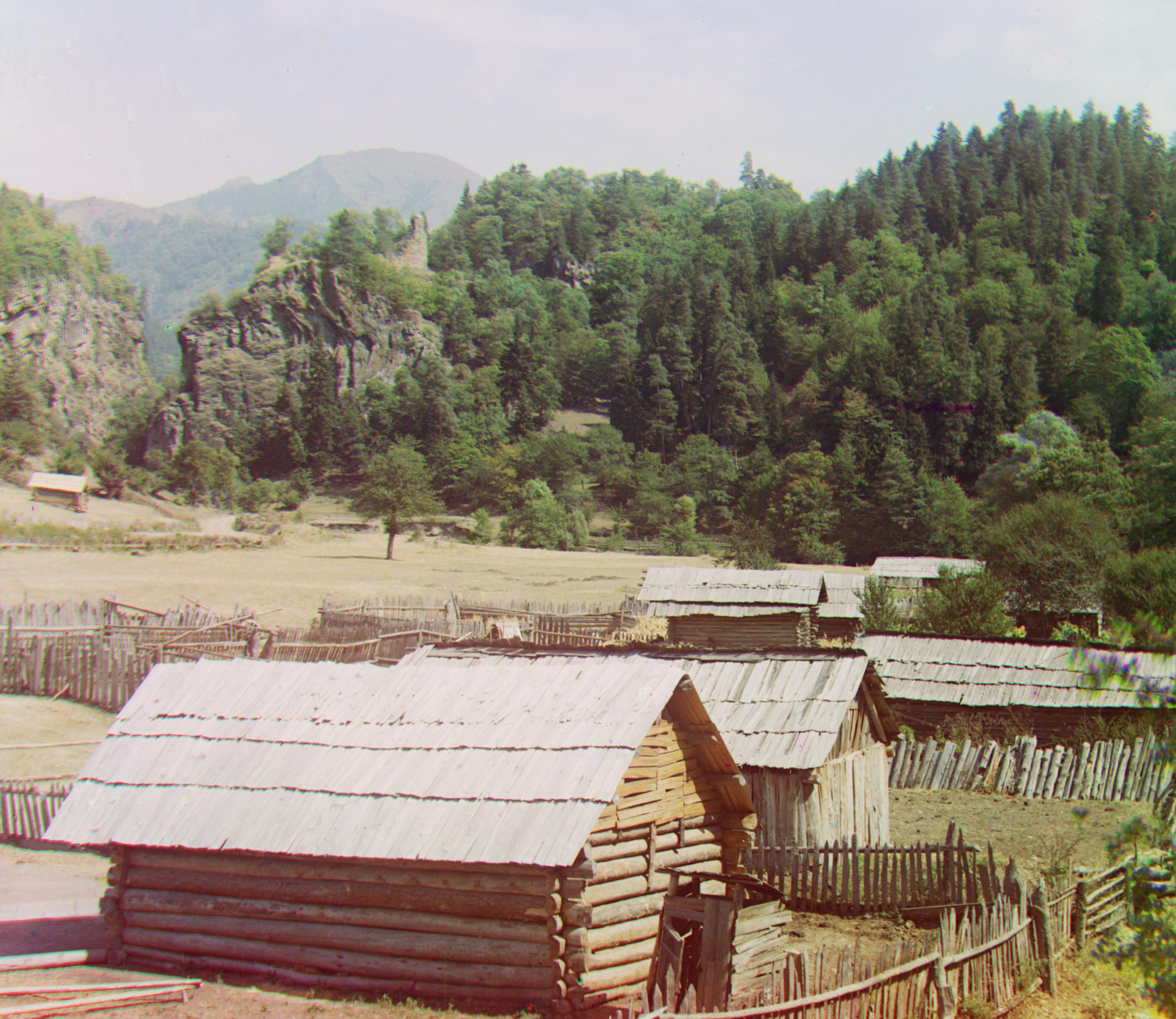
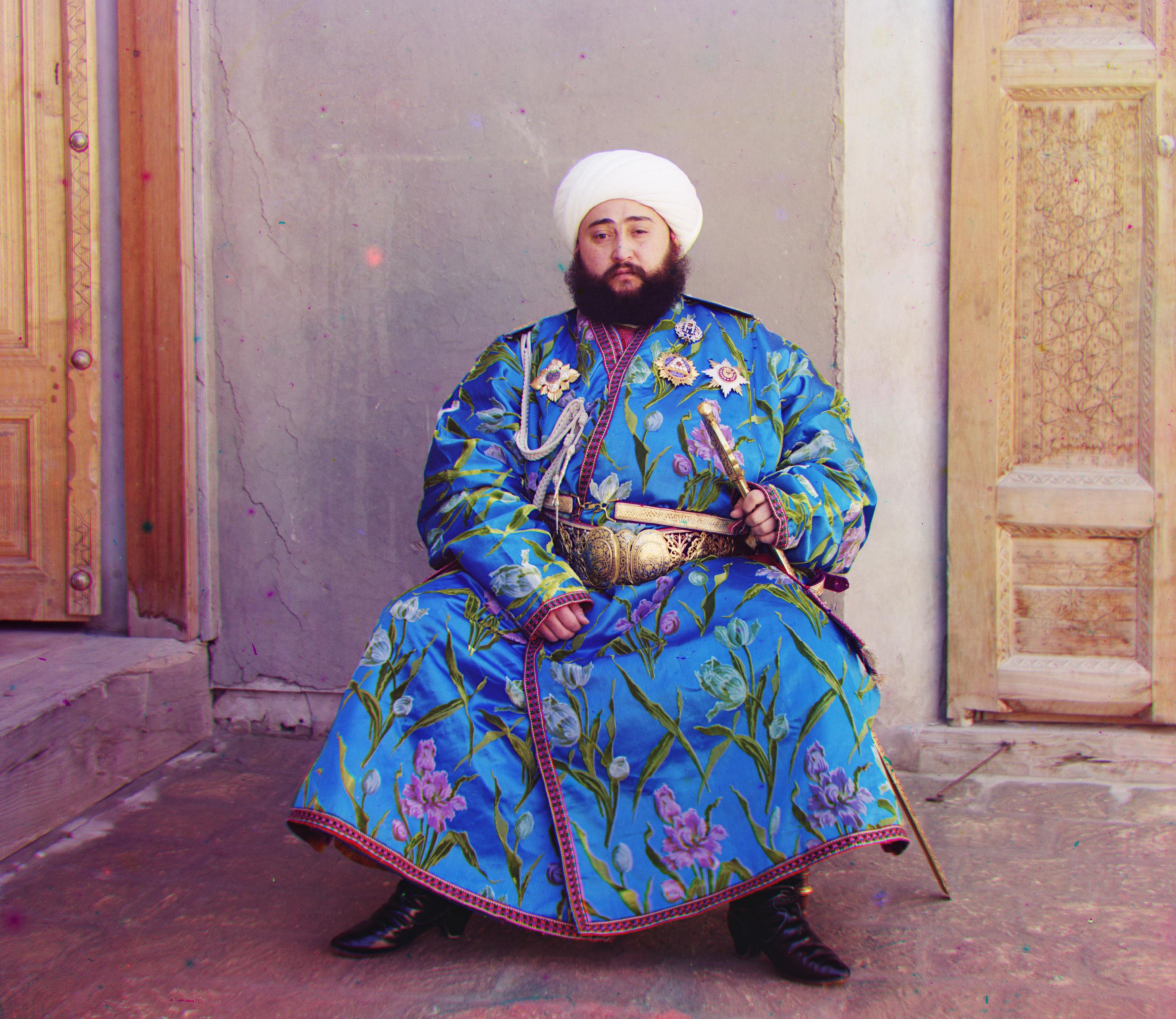
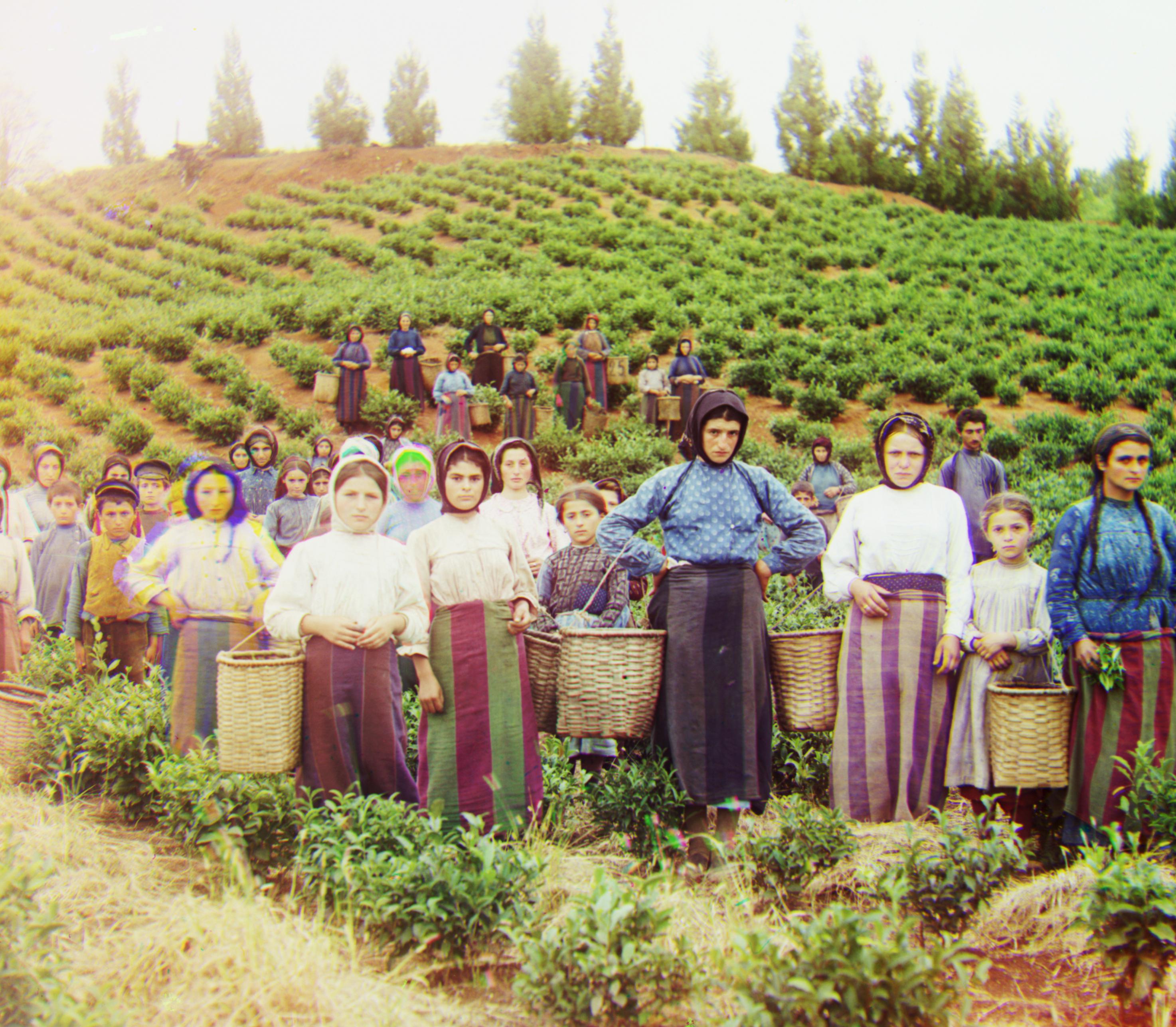
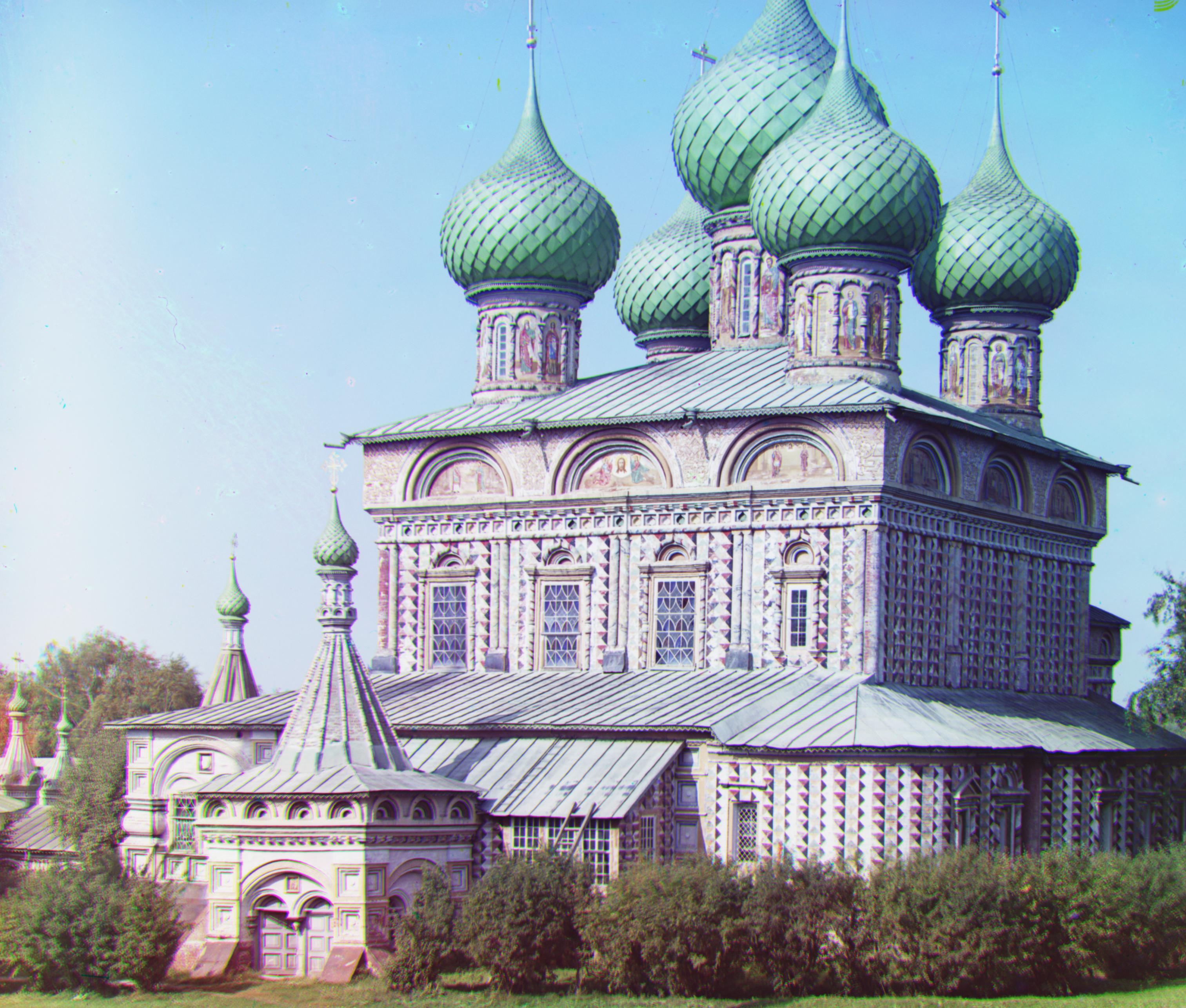
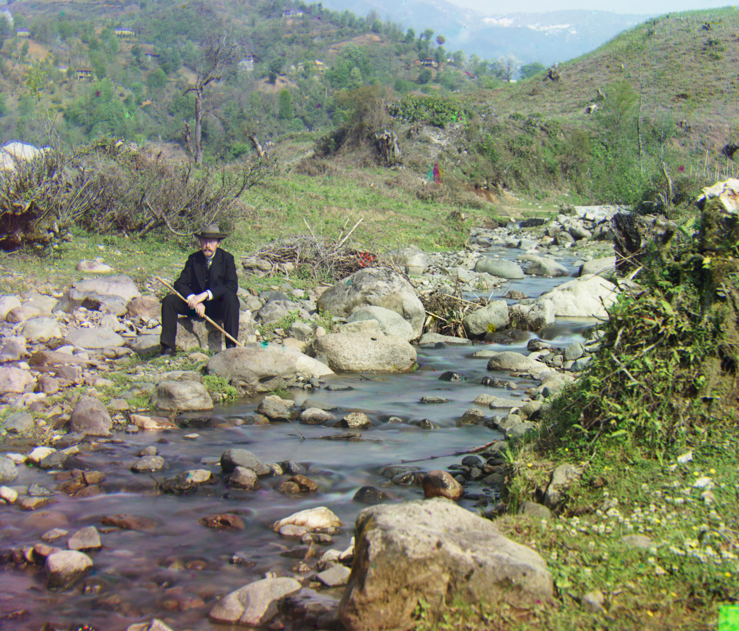
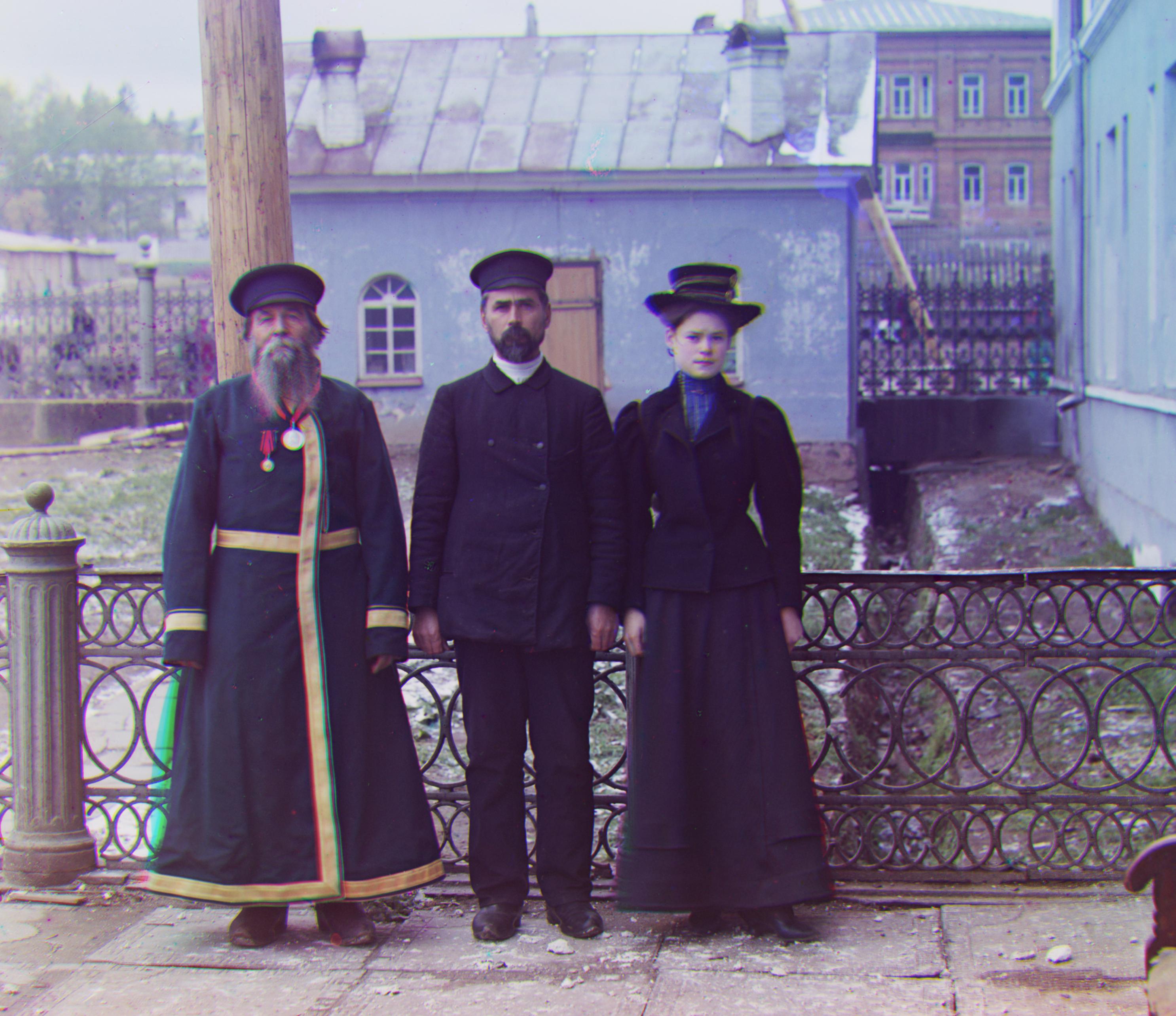
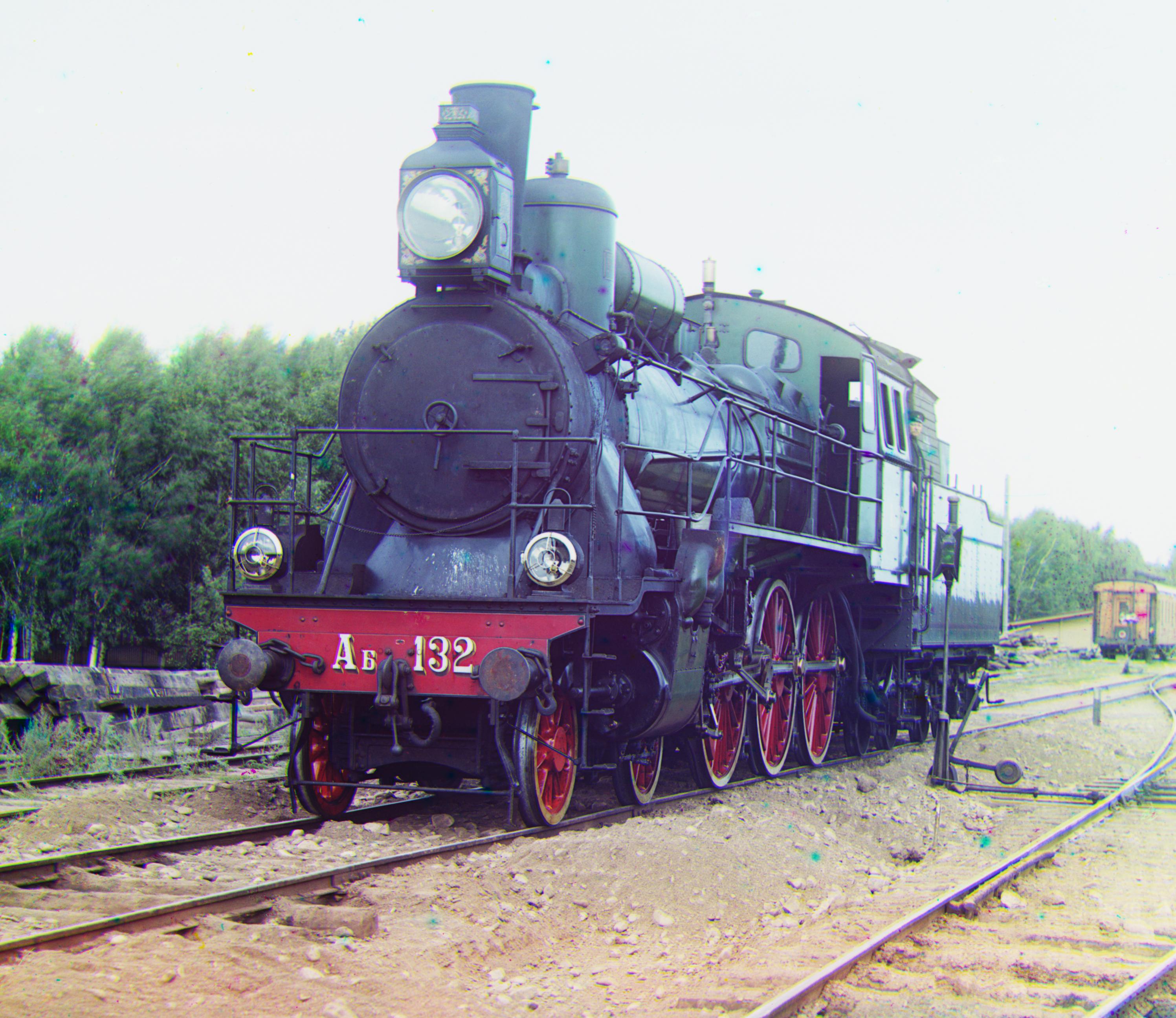
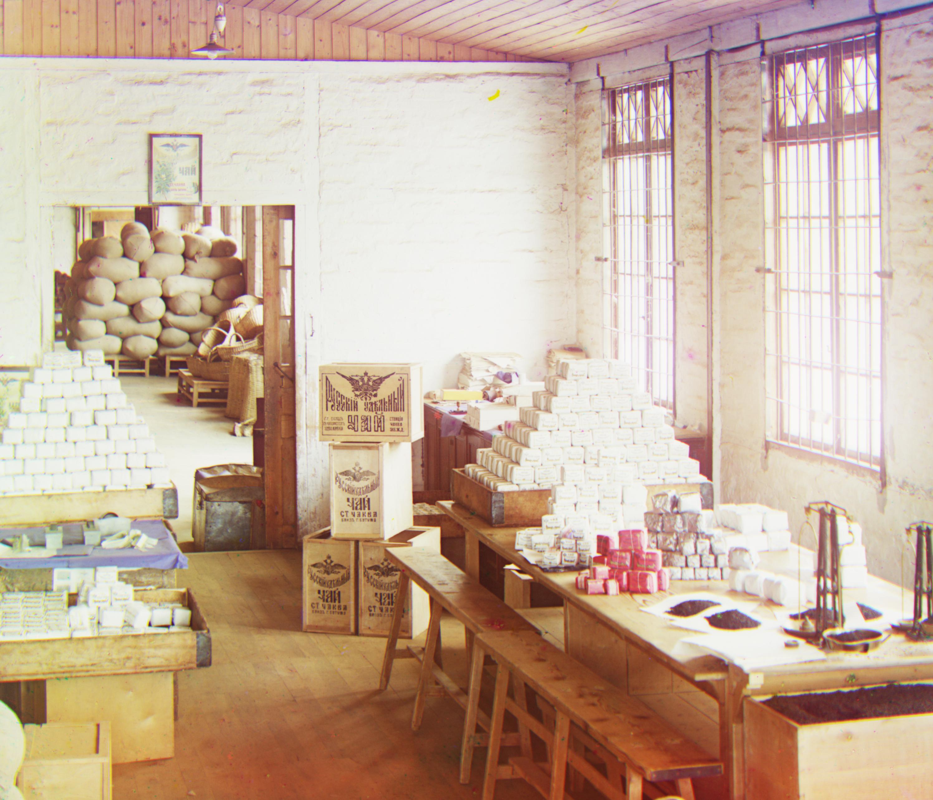
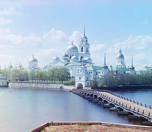
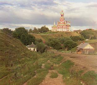
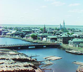
The goal of this project was to take these glass plate negatives (which indivdually appear as black and white pictures) and output the colored image. Essentially, this allows us to see exactly what Sergei saw when he took those pictures in Russia over 50 years ago.
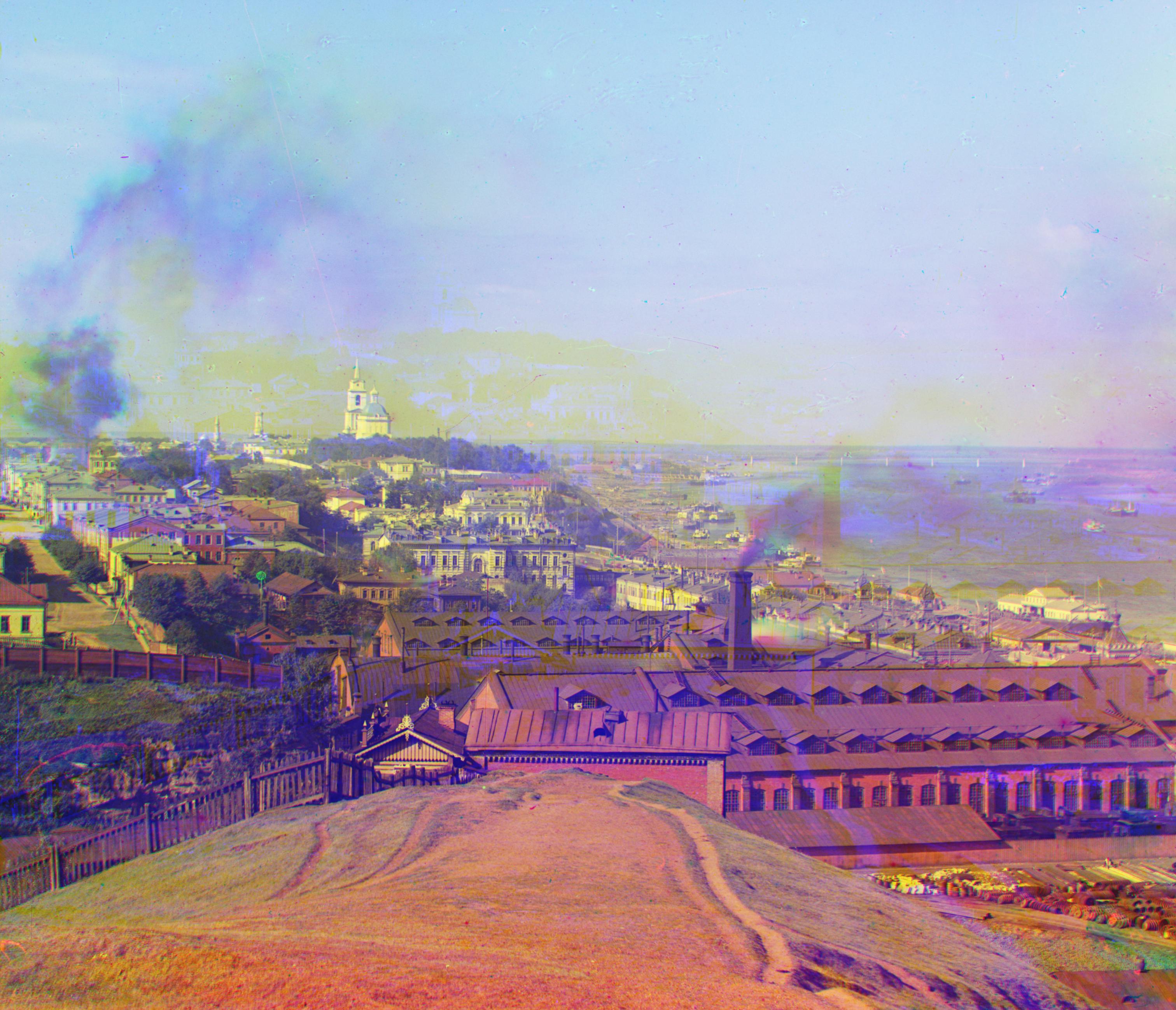
Combining these exposures enables us to see the original image in colorized form. Since he used a three-stack camera, each image has a slight offset in what it displays. This offset creates an obstacle because you can’t directly align the images on top of one another to retrieve the colored image. Therefore, we need to come up with an approach to deal with that offset.
My main approach for the smaller .jpg images is to crop one image and align the two other full images against the cropped image. By “align”, I mean exhaustively looking through the potential (x,y) starting positions where the cropped image could be placed on the full image and calculating the mse of the cropped image against the same overlapping region of the full image.
To begin, I cropped 10% from each edge of the green image, which means I would only calculate the mse in the middle 80% of each image. This helps because then the borders wouldn't interfere with alignment.
Then, I aligned this cropped green image against the full red image. The alignment returns the cropped section of the full red image for whichever alignment with the cropped green image produced the lowest mse. Then, I repeat this process with the cropped green image and the full blue image. Using the cropped green image and the aligned red and blue images, we create a complete colored image.

I ran into some issues with figuring out how to align the cropped green image against the full image. At first, I cropped the red and blue images and tried to align them against the base green image. This proved to be a more difficult approach because if the cropping cut off a significant part of the image, it would be harder to align the other images to the base.
For the bigger .tif images, I use the pyramid alignment strategy. The idea behind this strategy is to first find the correct alignment on a smaller version of the image, so that you can cut down the search space for later iterations where you are working with bigger images. This algorithm works better with bigger images, so you can save running time and memory.
This pyramid image layering strategy involves using a scaling factor to reduce the pixel size of the image in each layer. The bottom layer of each pyramid is the original image with the original pixel size. As you go up the pyramid, I use a scaling factor of 2 to reduce the pixel size of the image in each layer until I get to an image that has <= 50 pixels in width and height.
To begin, I took the highest layer (lowest number of pixels – blurriest image) and used the previous strategy to exhaustively search for the optimum starting (x,y) points. Then, we use those optimum starting points to create a range of where the starting point for the next layer could be. The reason this works is because I used a scaling factor of 2, so with each layer, I have double the number of pixels, which means double the number of potential starting (x,y) points.
For example if we find the optiumum starting point for the highest layer is at (1,2) , then the starting point could be between (0,2) and (2,6) in the next layer. Width: the new range for potential x starting points is between (1-1)*2 and ((1+1)*2). Height: the new range for potential y starting points is between (2-1)*2 and ((2+1)*2).
Instead of computing the mse for all the starting points, we instead compute it for the starting points within that range, which saves a lot of running time. We continune this process until we get to the bottom layer, which contains the original image. At that point, we have the optimum placement for the cropped green image against the full red and blue images so that the images line up properly. Using this placement, we create a colored image.