Fun with Filters and Frequencies

By Jay Shenoy

Part 1: Fun with Filters

Finite Difference Operator

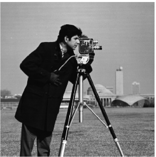
Image gradients provide a versatile tool for edge detection.

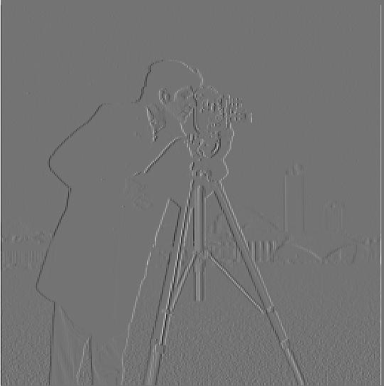
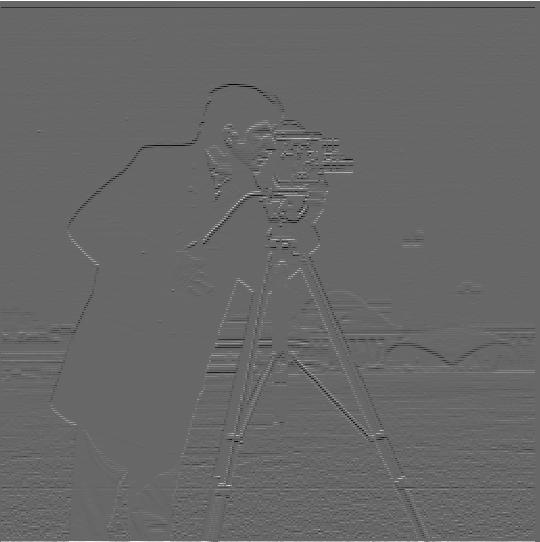
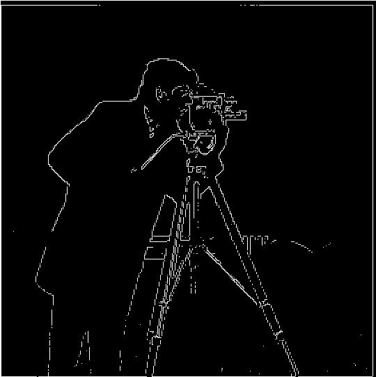
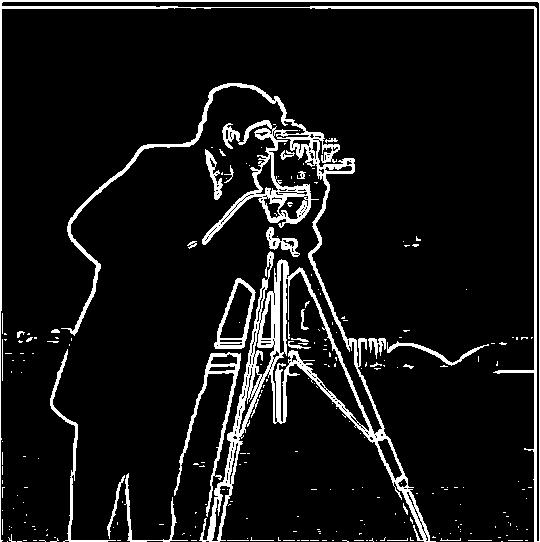
To compute the gradient magnitude of the cameraman image, I first computed the x- and y-gradient images. For the x gradient, I convolved the image with the single-row finite difference operator [1, -1]. For the y gradient, I convolved the image with the two-row, single-column difference operator [[1], [-1]]. These operators effectively compute the intensity difference between consecutive pixels in the x- and y-dimensions. The squared magnitude of the gradient vector at each pixel is the sum of the squares of the x- and y-gradients at that pixel, as computed previously. Since the magnitudes are relative, using the squared magnitude is sufficient for visualizing the gradients.

Part 1.2: Derivative of Gaussian (DoG) Filter

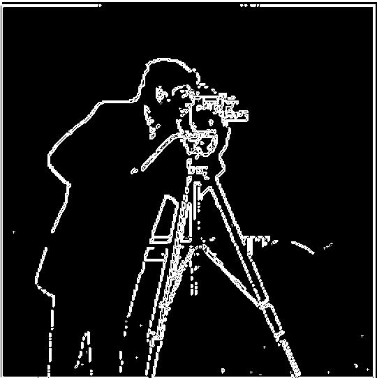
The edge image produced from the gradient magnitudes previously is noisy. To alleviate this issue, I convolved the image with a Gaussian blur filter before computing the gradients. The new edge image is shown below:

The gradient magnitude image seems less noisy and the edge lines are more solid than before. This is because the image of the cameraman is blurred before we take the gradients, meaning that any high-frequency noise is filtered out. This noise previously caused thin, choppy lines in the gradient magnitude image, which are no longer present.

One can also combine the Gaussian blur with the gradient computations into two standalone filters, thanks to the associative property of convolution. The resulting Derivative of Gaussian (DoG) filters are visualized below:

By convolving the cameraman image with two DoG filters, we get virtually the same edge image as before (shown below).

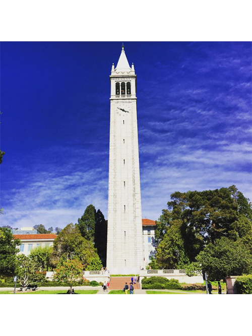
Part 1.3: Image Straightening

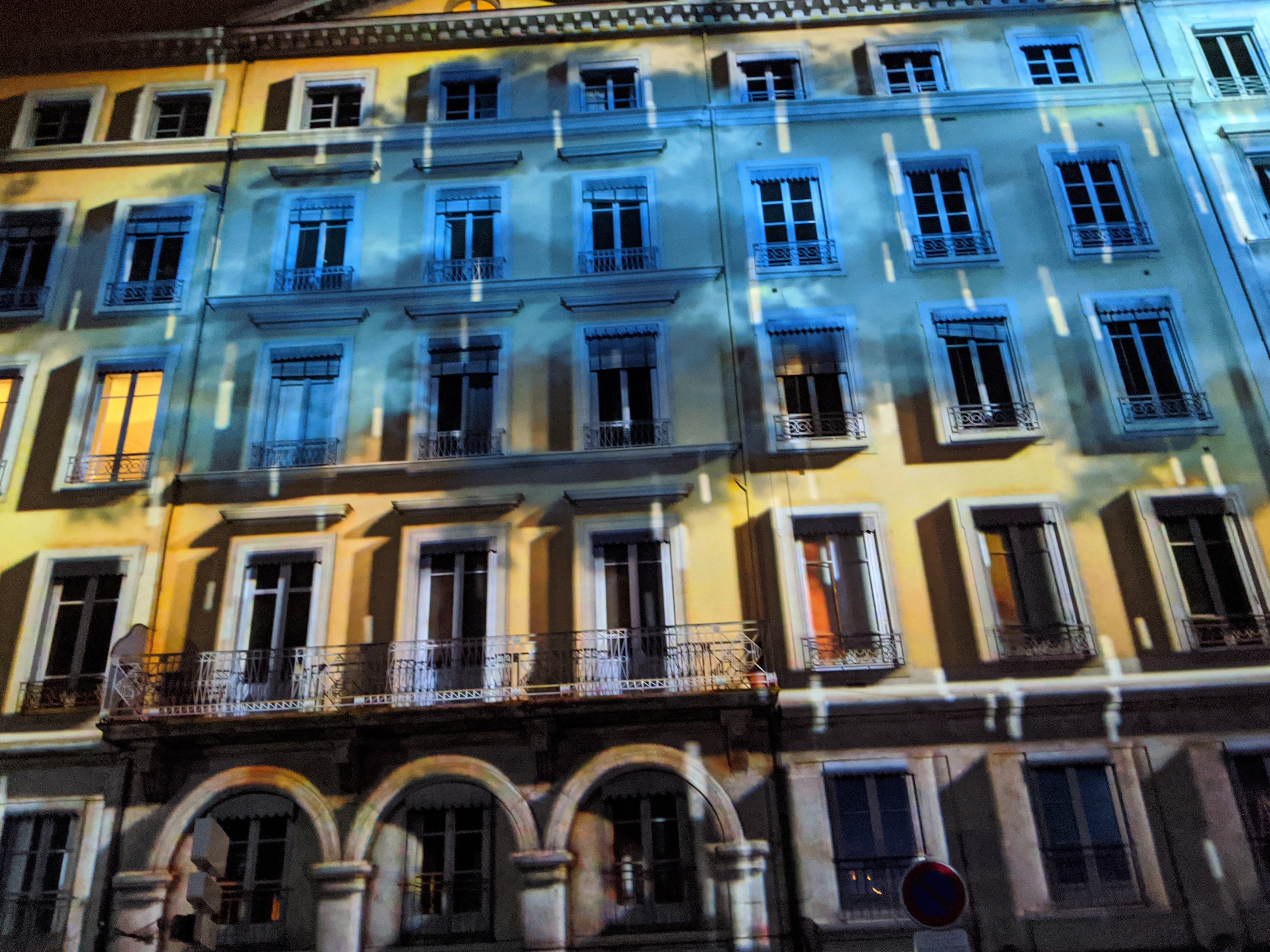
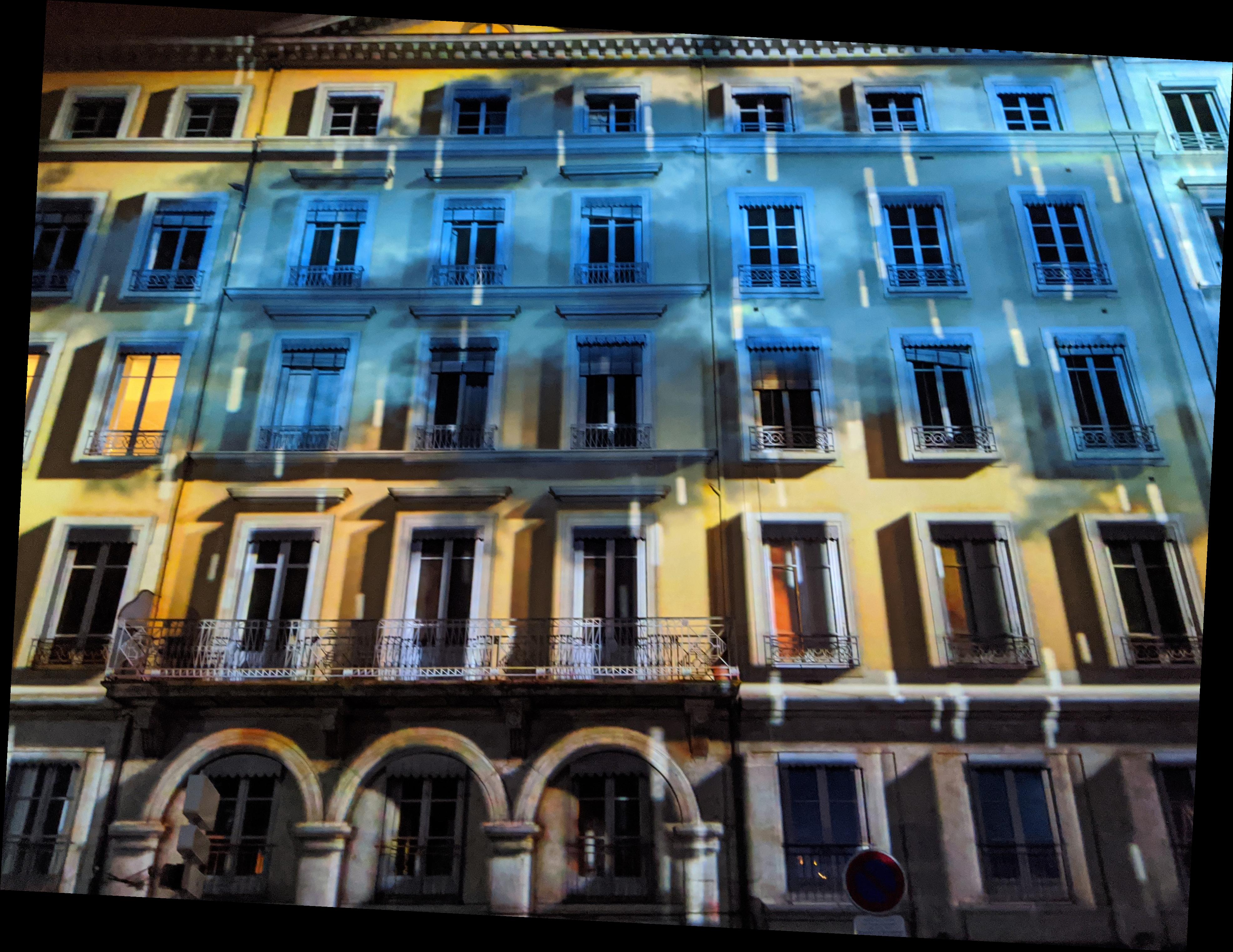
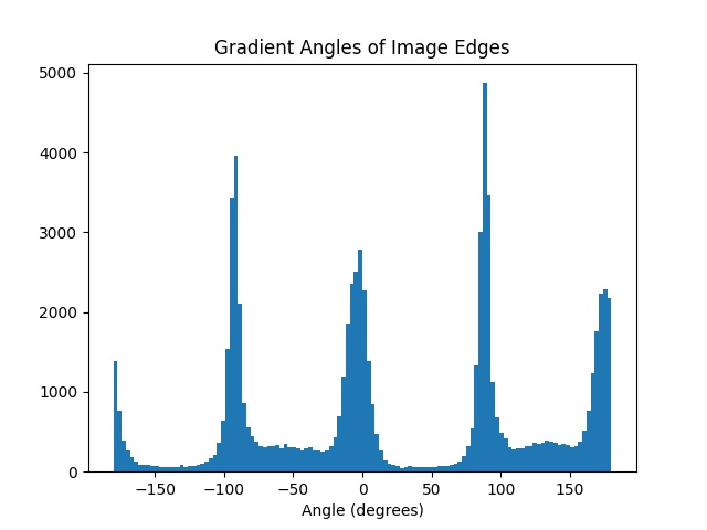
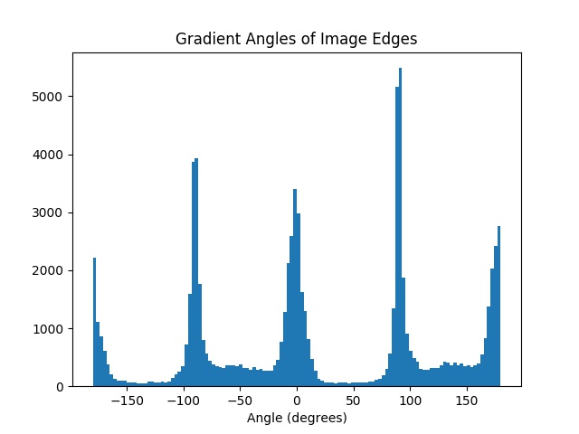
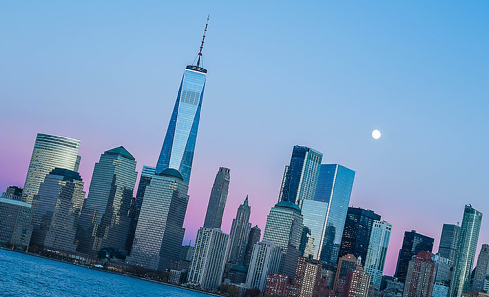
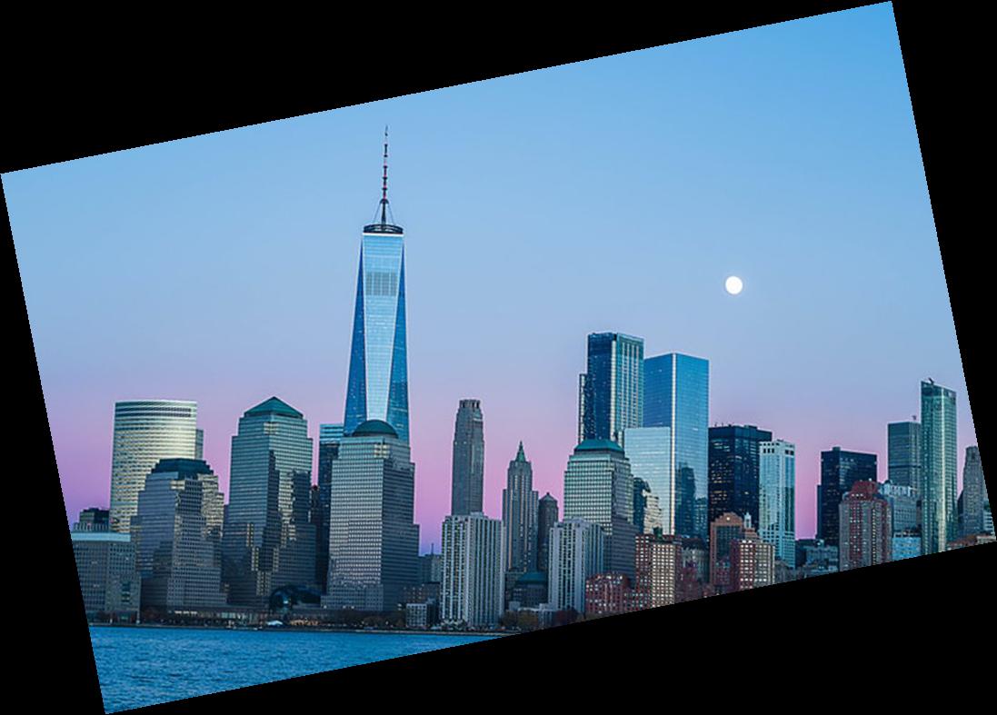
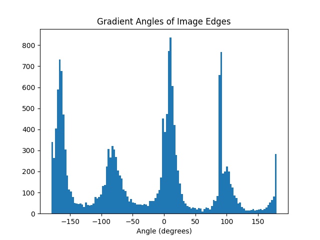
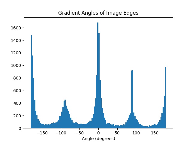
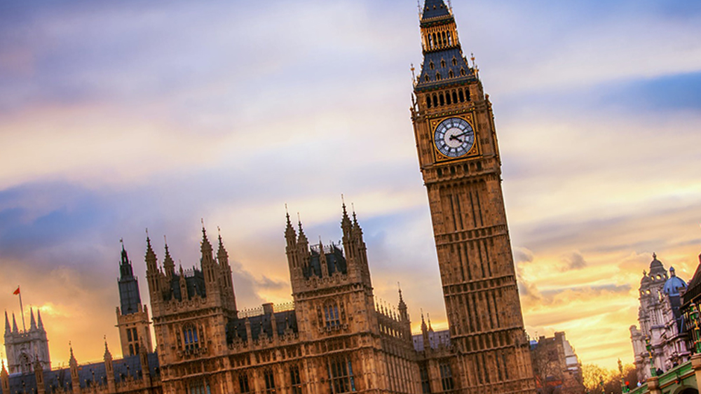
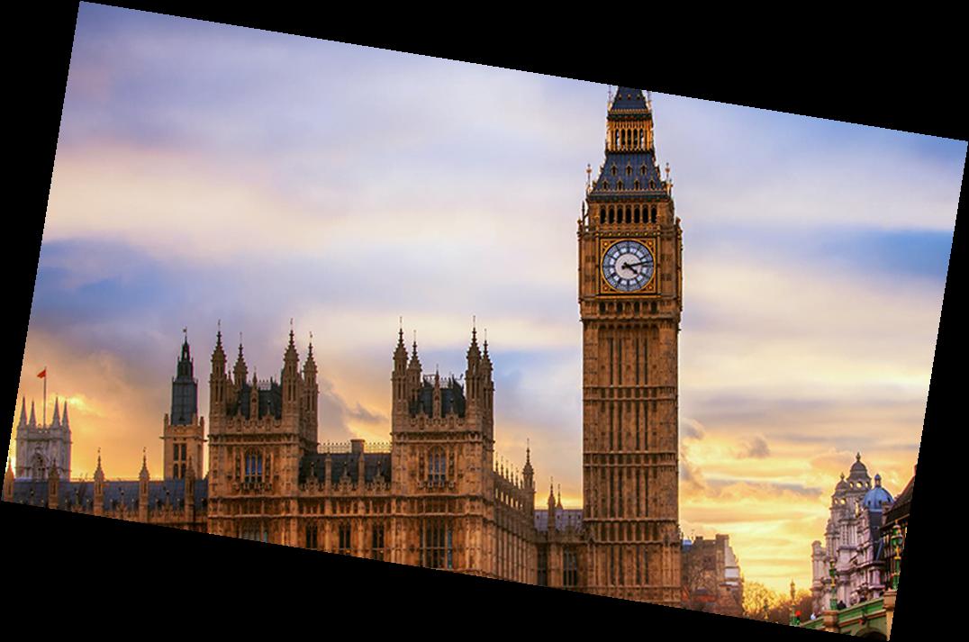
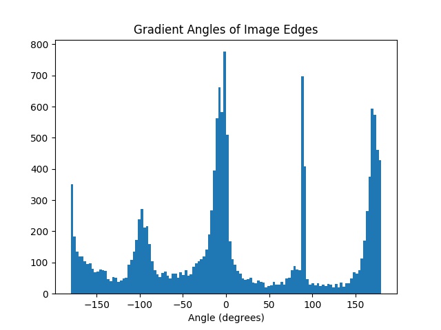
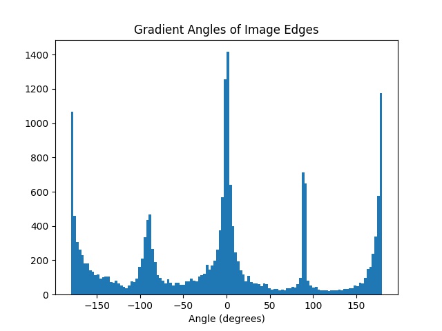
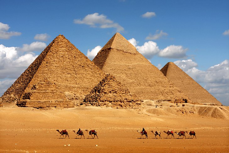
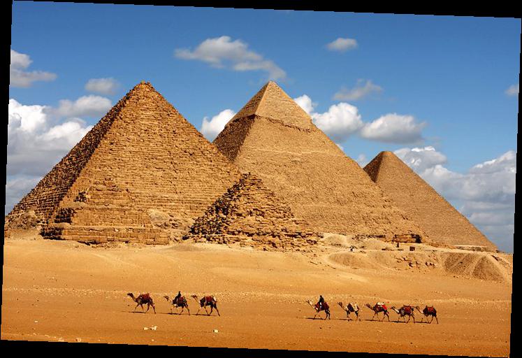
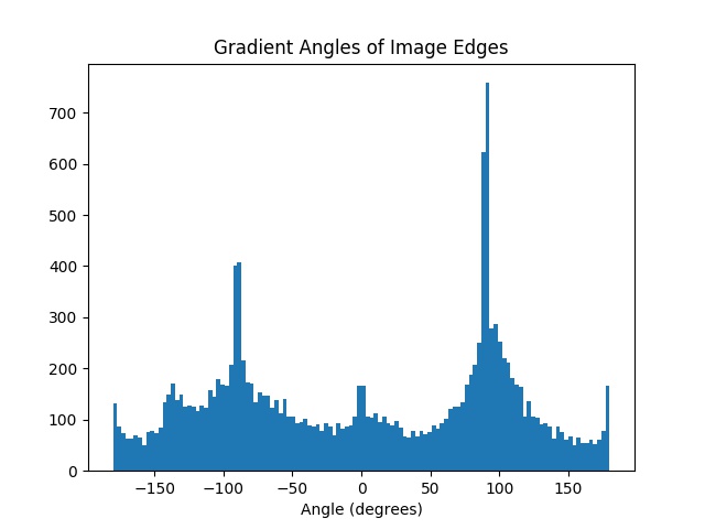
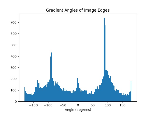
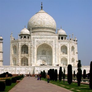
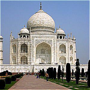
Photos we take are often not straight. To fix this, I implemented a straightening algorithm that attempts to maximize the proportion of vertical and horizontal edges present in the image using the previous DoG filters. This algorithm relies on the assumption that most pictures primarily contain vertical and horizontal edges due to gravity. The straightness of an edge is computed using the angle of the gradient vector at each pixel (the inverse tangent of the y-gradient over the x-gradient). The results of the algorithm are shown for four images below, along with the orientation histograms of the gradient angles:

As you can see, the straightening algorithm fails when applied to the last image of the Pyramids of Giza. The original image is perfectly straight, but because the gradient angles are distributed more uniformly than for the other images (seen from the orientation histogram), optimizing for vertical and horizontal edges fails in this case. As a result, the algorithm tries to rotate the image even though no straightening is necessary.

Part 2: Fun with Frequencies

Part 2.1: Image "Sharpening"

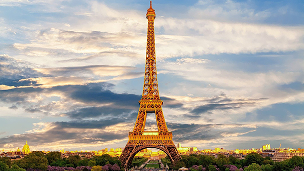
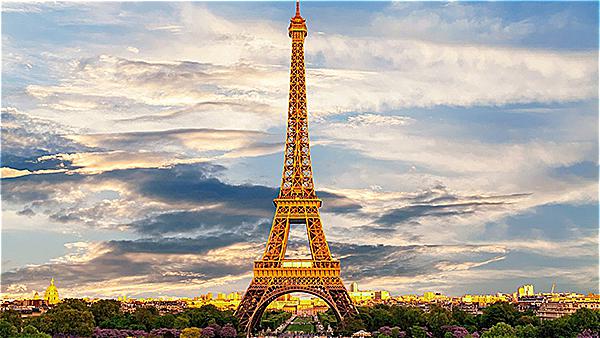
To sharpen images, I implemented the unsharp mask filter, which essentially applies a high-pass filter to the image, and adds back a weighted version of the high-frequencies to the original image. This is done using a single convolution with what is known as the unsharp mask filter. Some results are shown below:

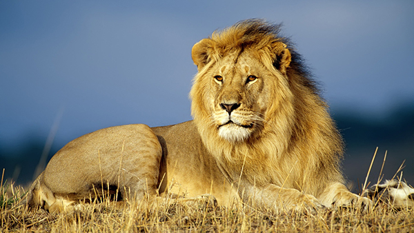
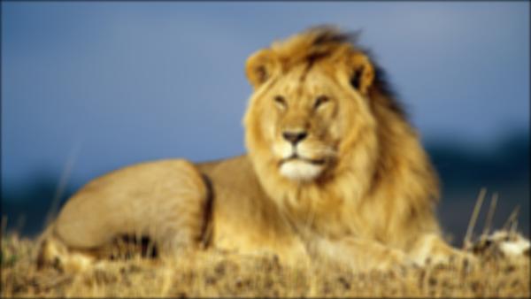
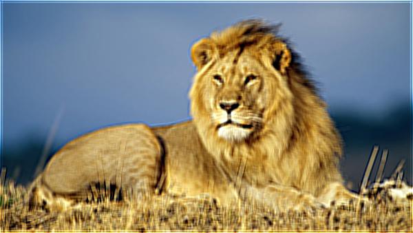
To test the efficacy of this pseudo-sharpening algorithm, I took a sharp image of a lion, blurred it, and then applied the sharpening algorithm. As you can see below, the sharpened image doesn't look the same as the original, but it indeed looks "sharper" than the blurred version.

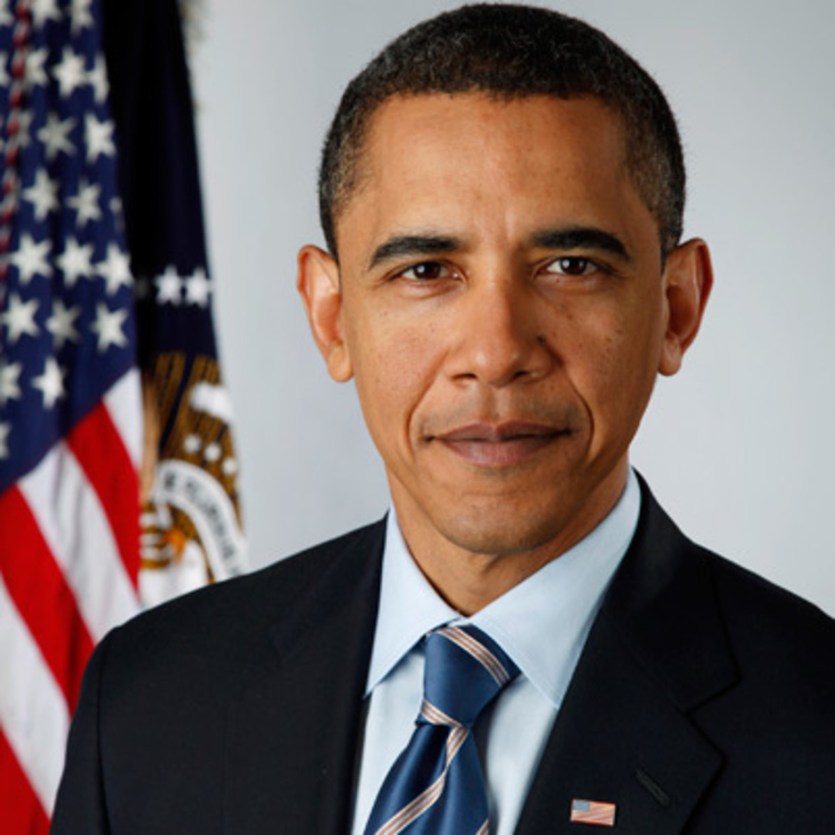
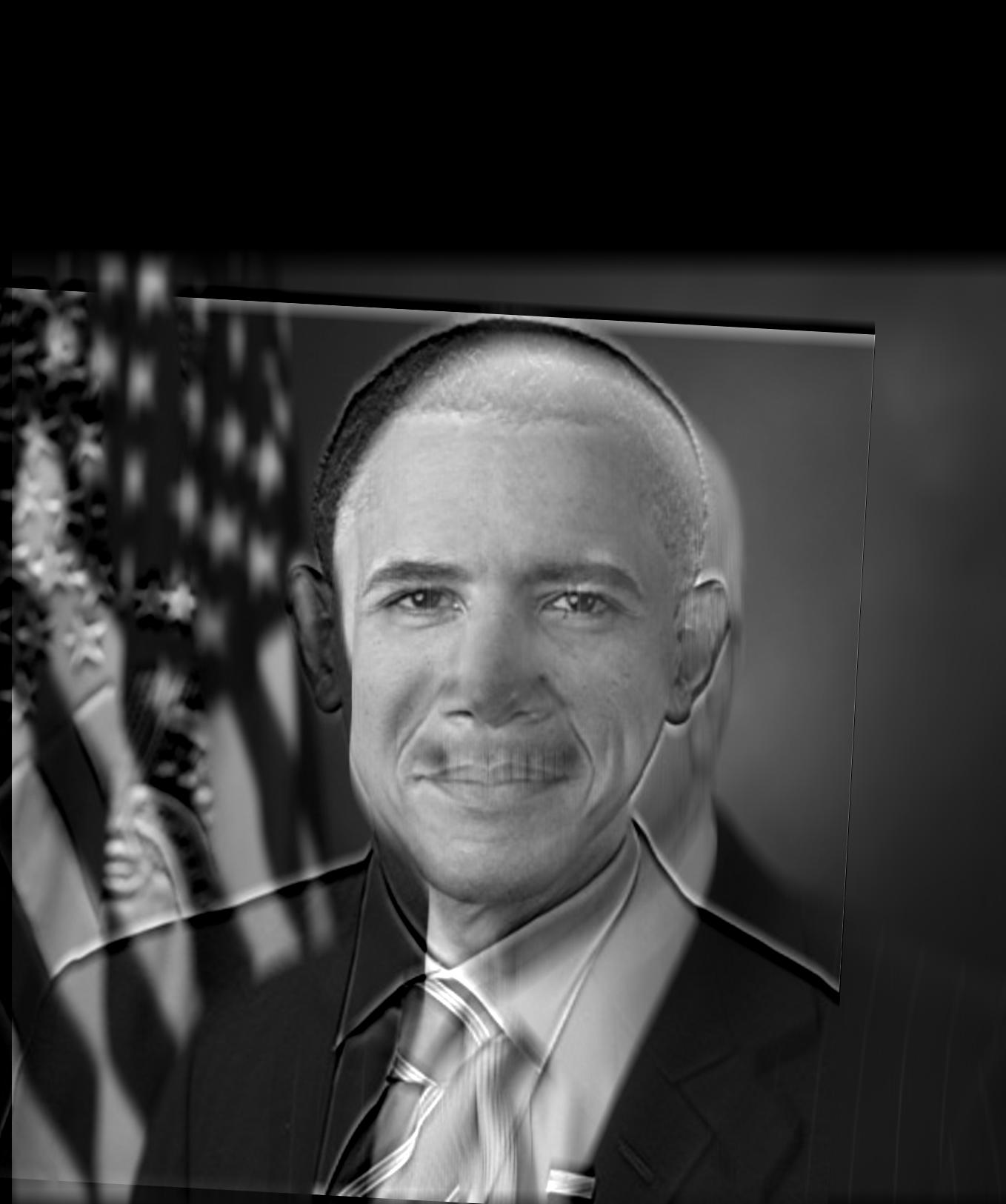
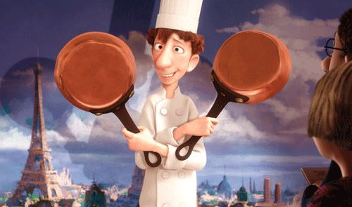
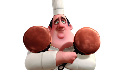
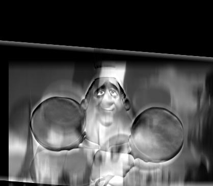
Part 2.2: Hybrid Images

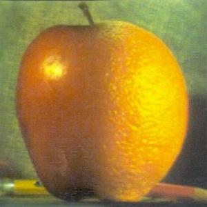
I implemented a technique that combines two images into a hybrid picture that looks different when viewed close-up vs. far away. This is done by low-pass filtering the first image, high-pass filtering the second, and combining the two to get a hybrid. Some results are shown below:

As you can see, the hybridization algorithm fails for the last image because it's difficult to find good cutoff frequencies for the filters such that we preserve sufficient low-frequency features for the image of Linguini while still being able to discern the high-frequency features of Gusteau.

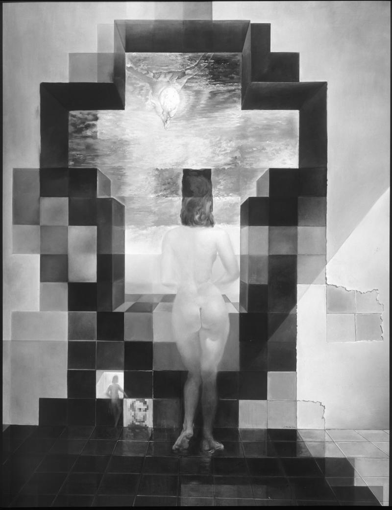
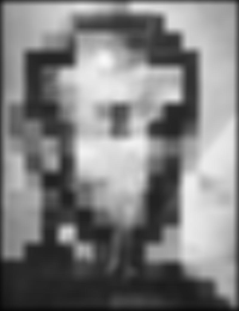
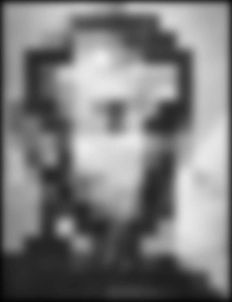
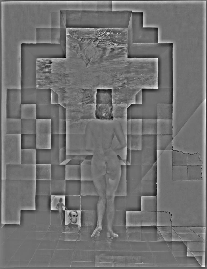
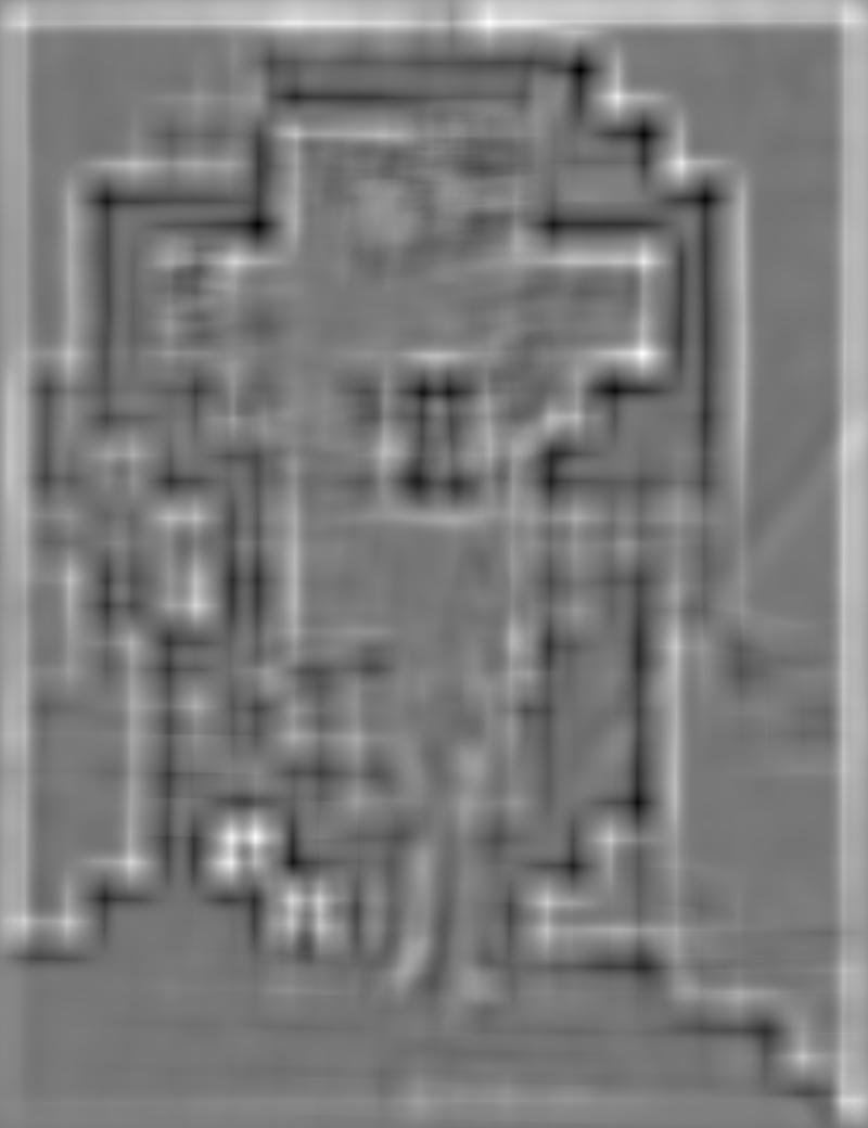
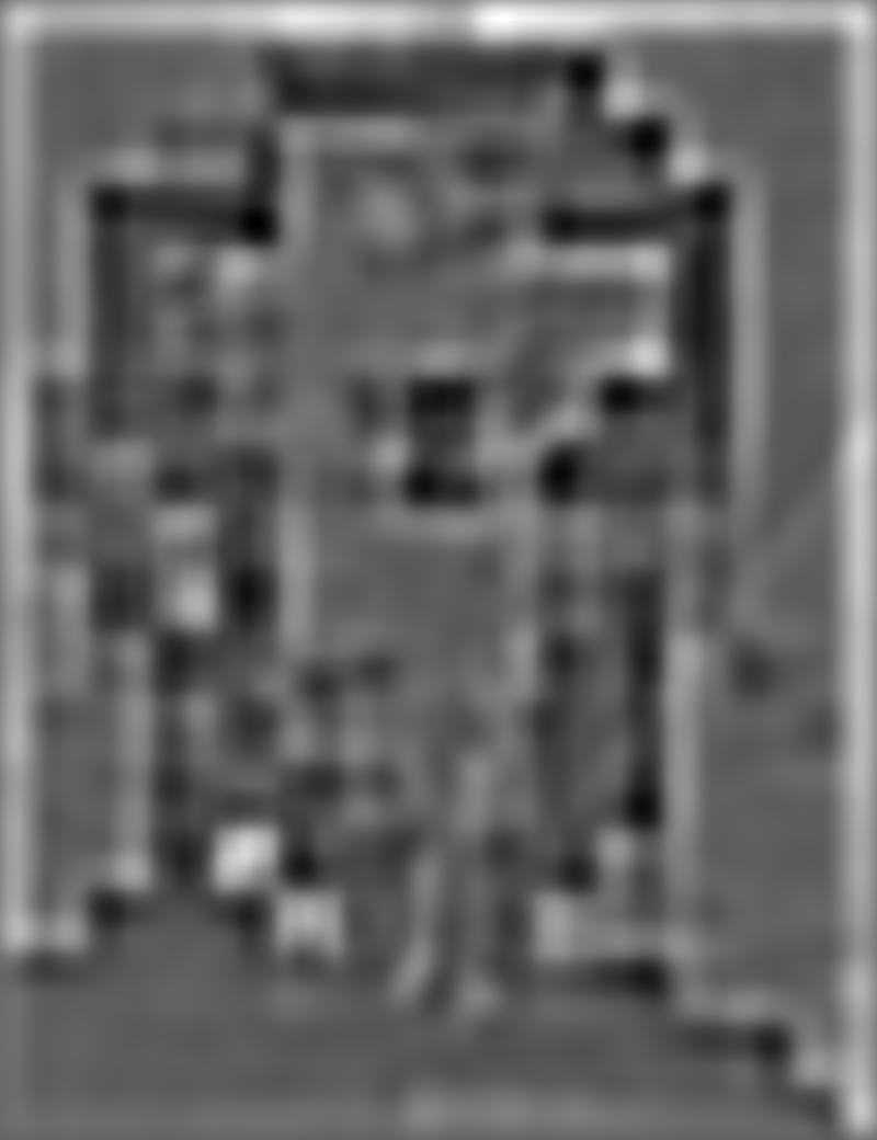
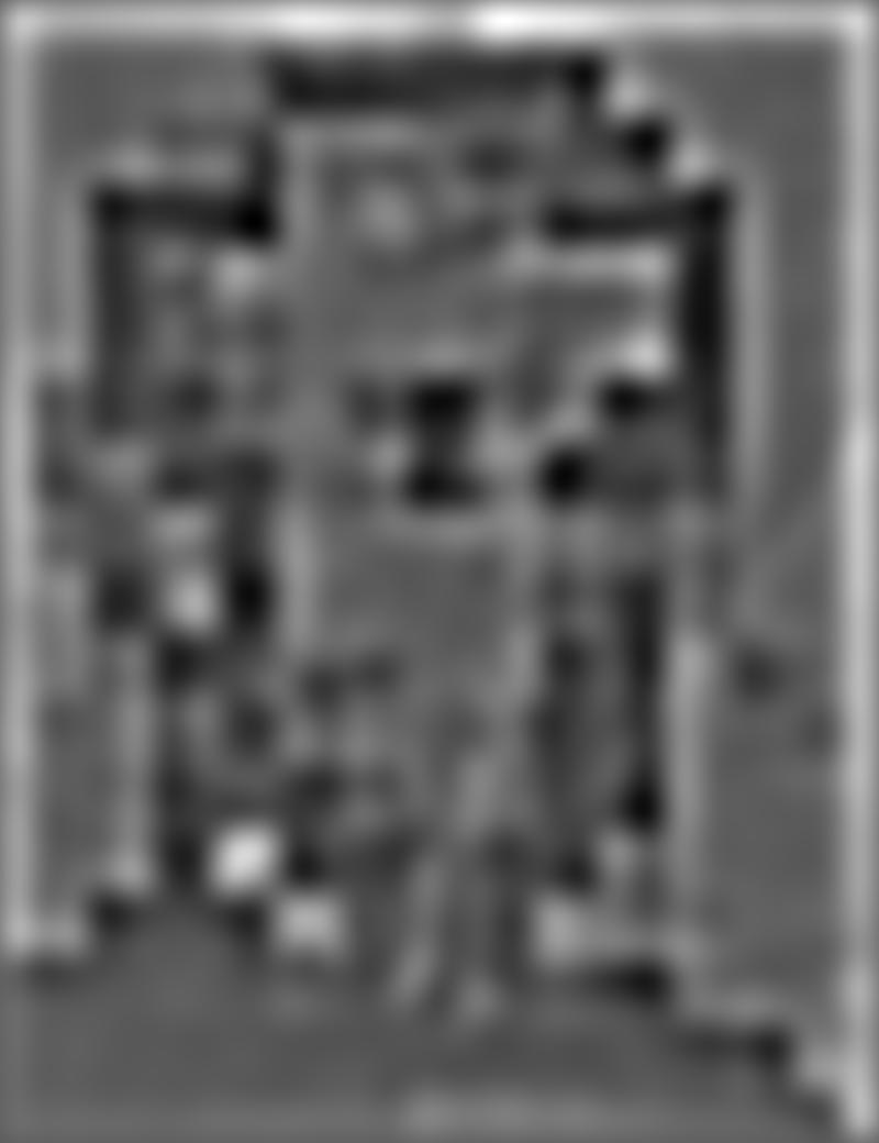
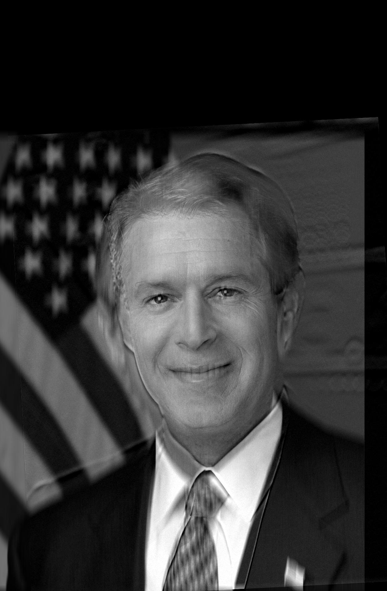
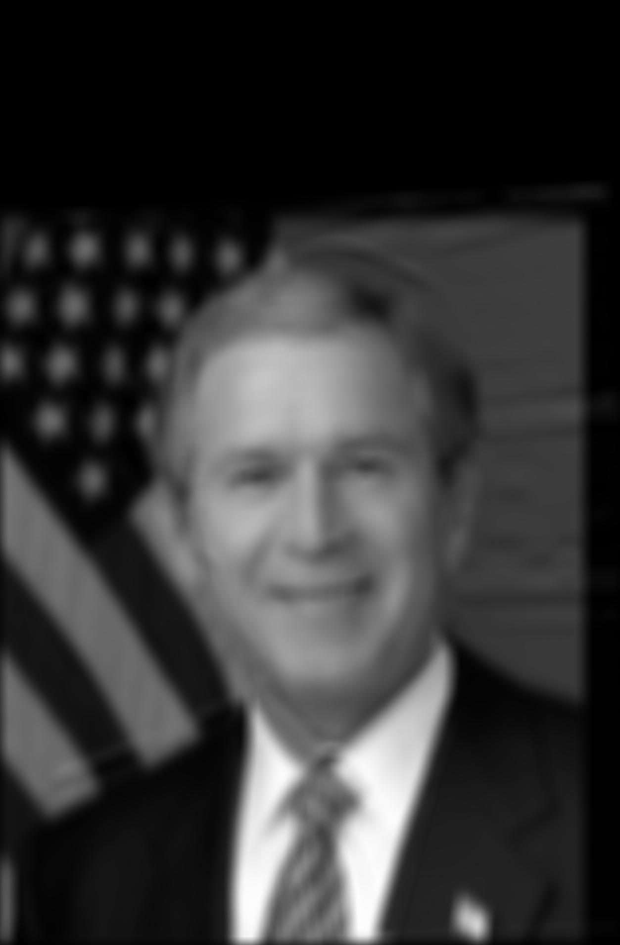
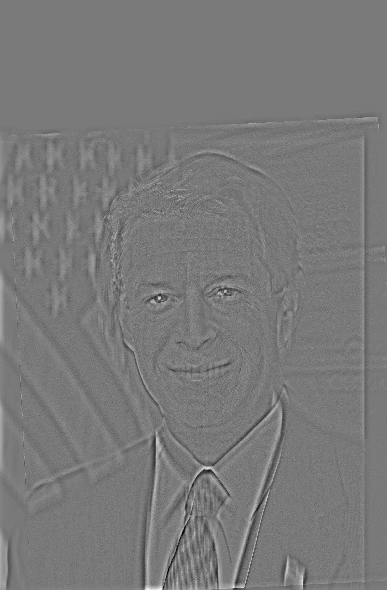
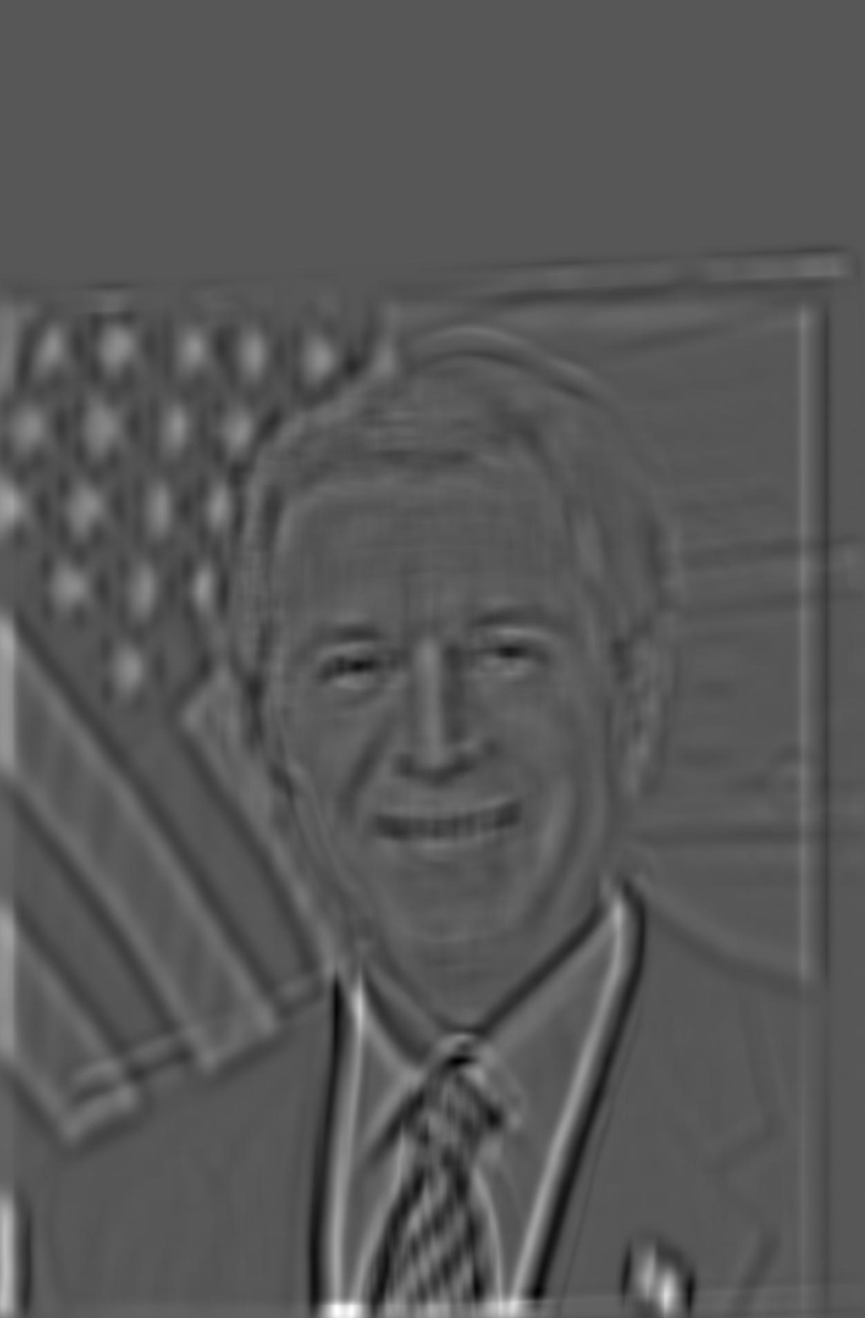
Part 2.3: Gaussian and Laplacian Stacks

Two important data structure used in image processing are the Gaussian stack and the Laplacian stack. Each level of the Gaussian stack applies a Gaussian blur to the level before it, starting from the original image. Thus, as we ascend the Gaussian stack, we only see frequencies of the image that are below a certain cutoff, and these cutoffs decrease for higher levels.

The Laplacian stack is related to the Gaussian stack in that each level is calculated by subtracting the corresponding level of the Gaussian stack with the next level (containing lower frequencies). Thus, the zeroth level of the Laplacian stack contains all frequencies from the original image between f0 and f1, the first level contains all frequencies between f1 and f2, and so on, where f0 > f1 > f2. The result is that each level of the Laplacian stack contains a band of frequencies.

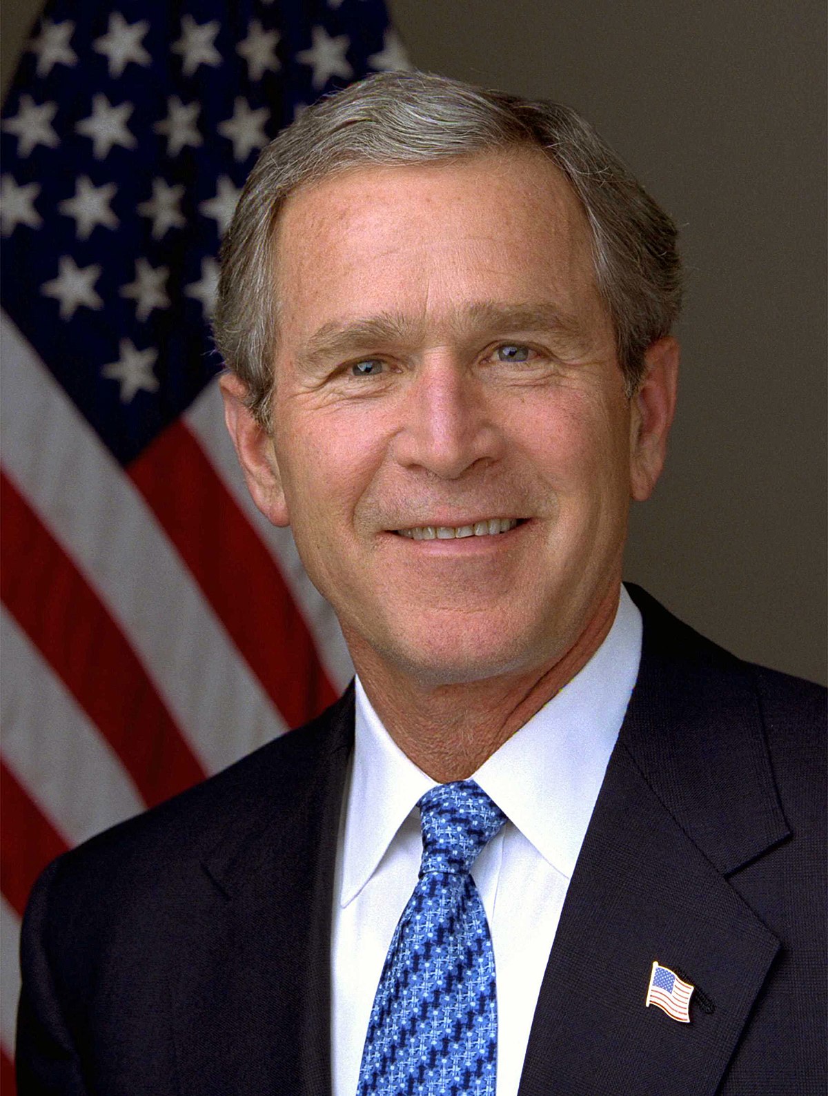
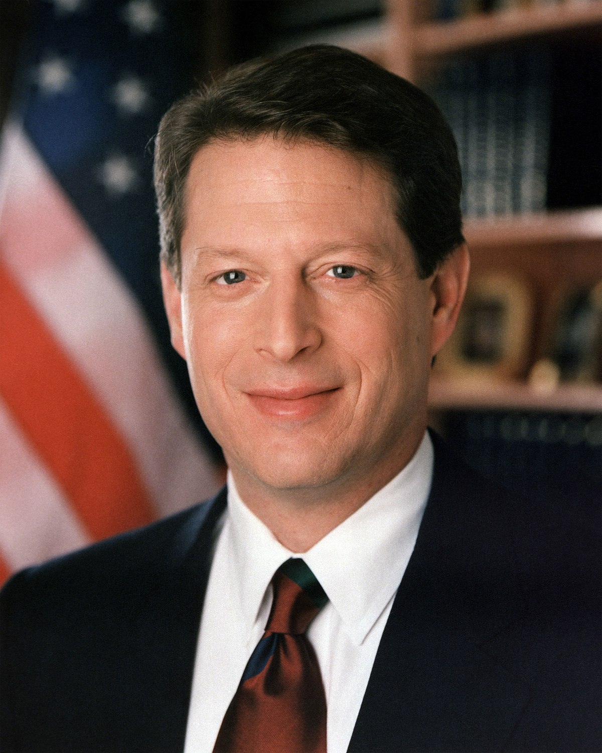
Gaussian and Laplacian stacks for a Dali painting as well as the Bush/Gore hybrid image from the previous section are shown below. These reveal the frequency content of the original images.

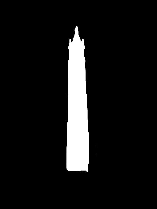
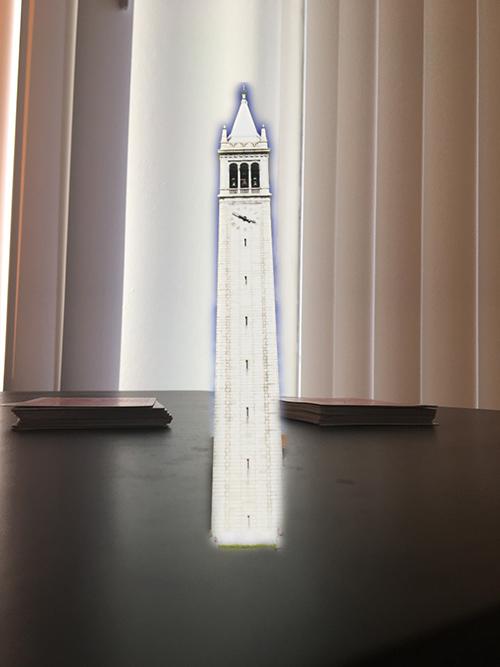
Part 2.4: Multiresolution Blending

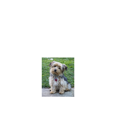
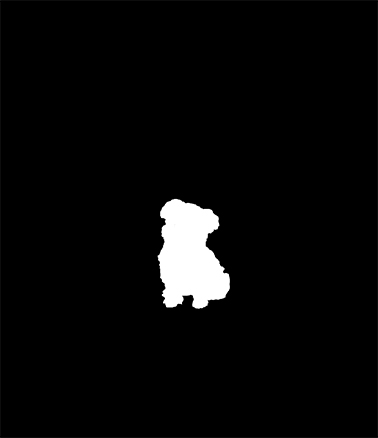
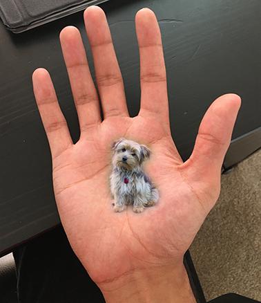
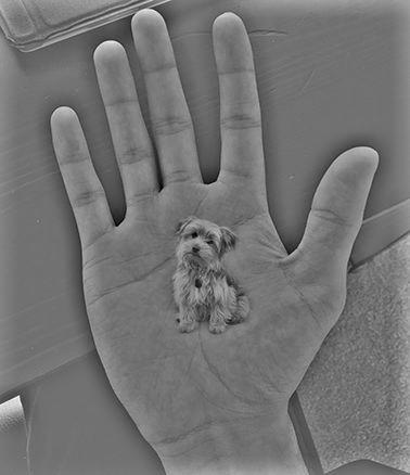
In part 2.2, we hybridized images by separating the input images into low and high frequencies and summing these two filtered photos. In this section, we blend two images together using a mask that separates the content of one image from the other. The images are blended by first calculating the Laplacian stacks of both, computing a Gaussian stack for the mask region, then blending the images at each Laplacian level using the corresponding blurred mask level for the blend weights. This creates a Laplacian stack for the blended image, which is summed to produce a final blended picture.

Some results are shown below:

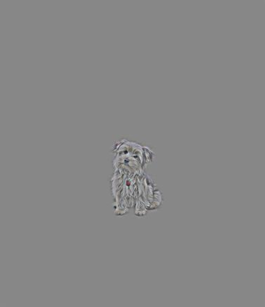
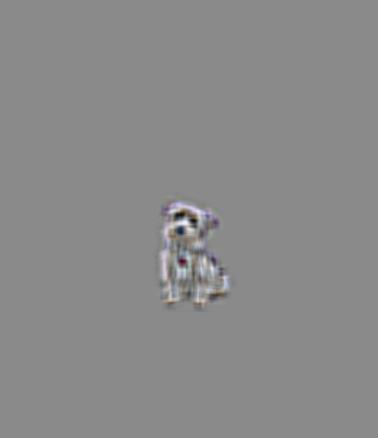
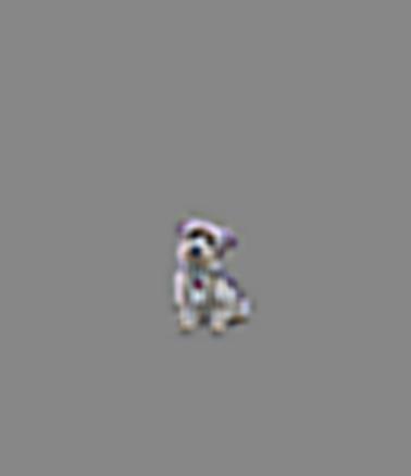
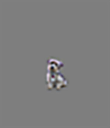
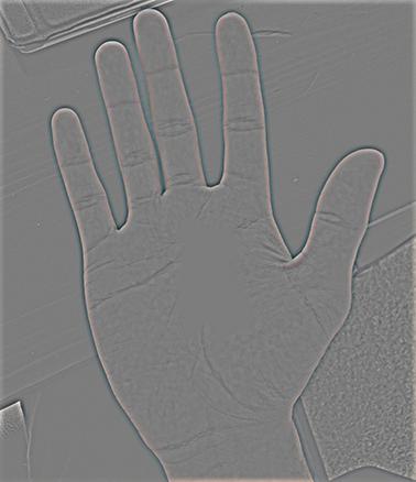
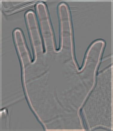
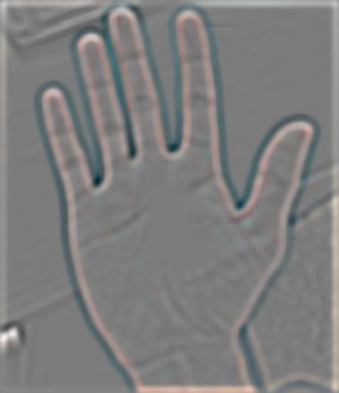
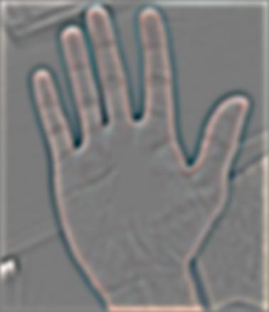
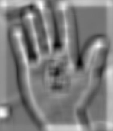
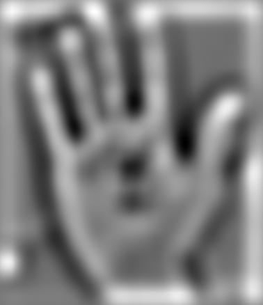
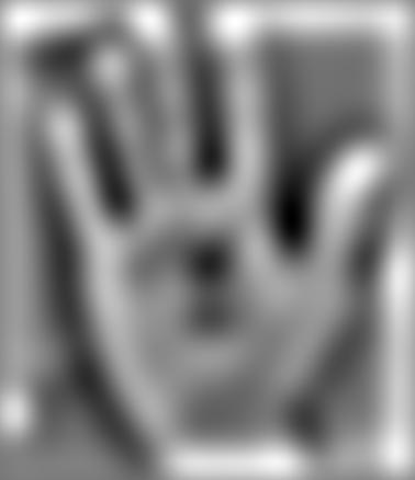
The Laplacian stacks for the masked dog, masked hand, and blended images are shown below.

Reflection

The coolest thing I learned while doing this assignment was how to properly do multiresolution blending. The problem of seamlessly compositing two images is doubtlessly one of the fundamental tasks in image processing, and I was surprised to see that a conceptually simple and intuitive technique like multiresolution blending was able to produce great results. The idea of applying a Gaussian blur to a mask image in order to determine the spline weights was new to me, and it proved to be particularly effective.