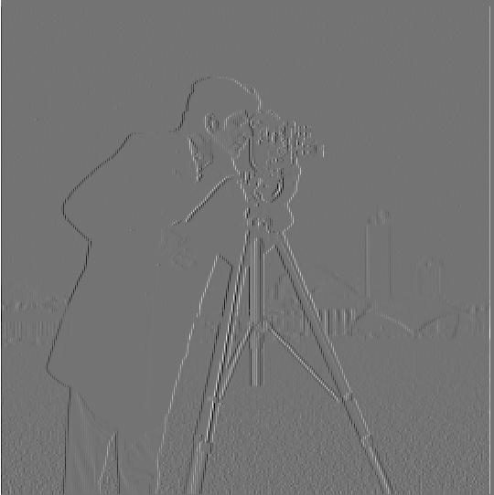
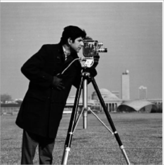
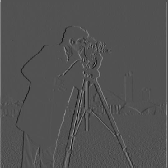
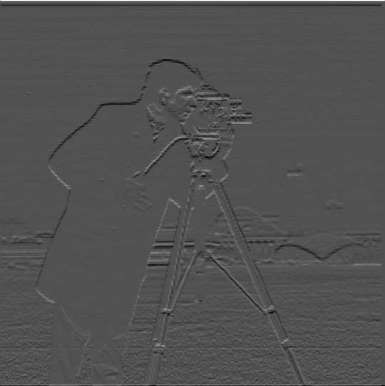
We study the finite difference operator following image, beginning with the vertical and horizontal directions, then taking the magnitude:
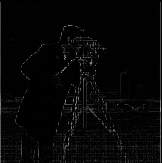
With the following results:
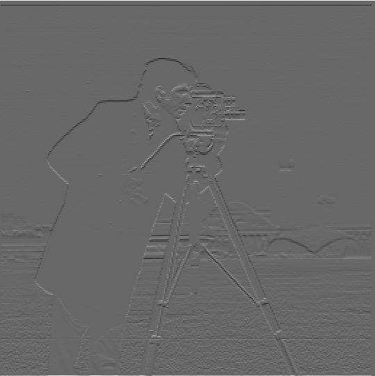
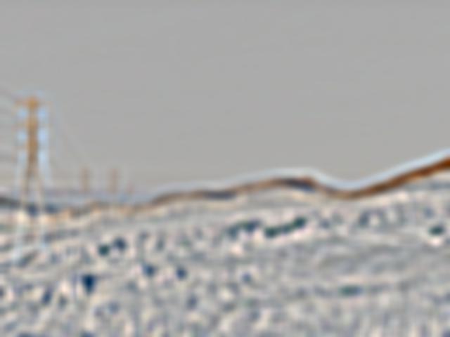
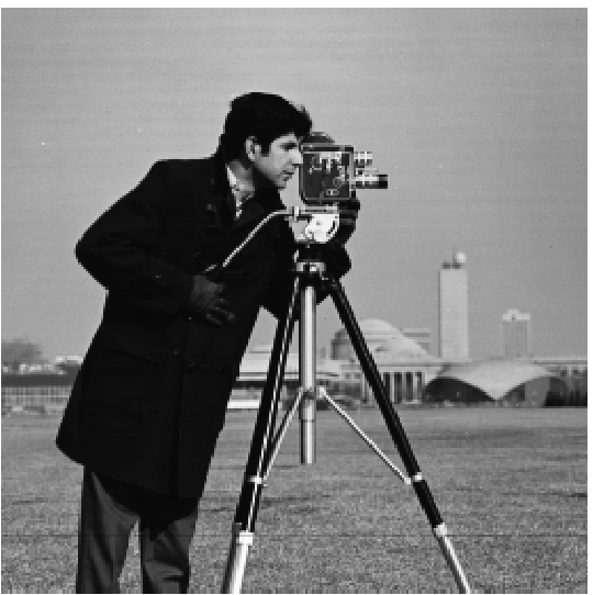
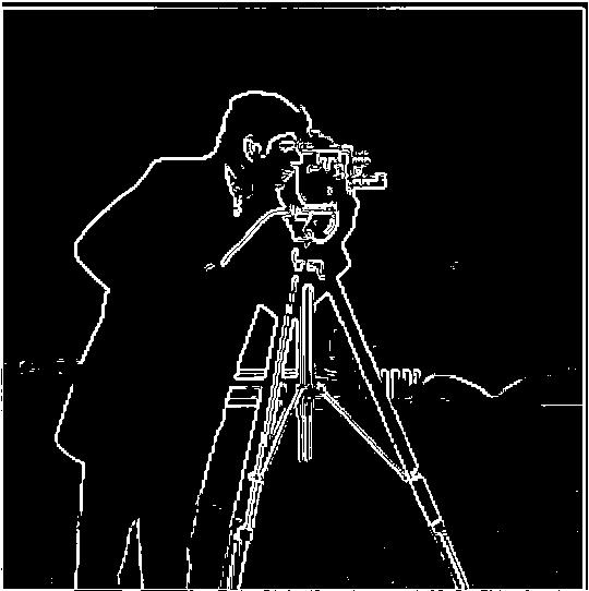
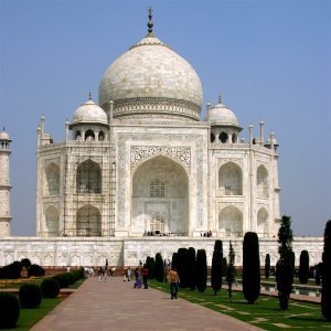
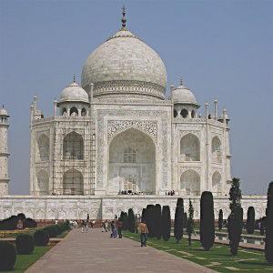
Now we try with the blurred cameraman image below. Note that the image is blurred, but it is difficult to tell on this writeup because the image is shrunk to be displayed here.
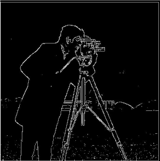
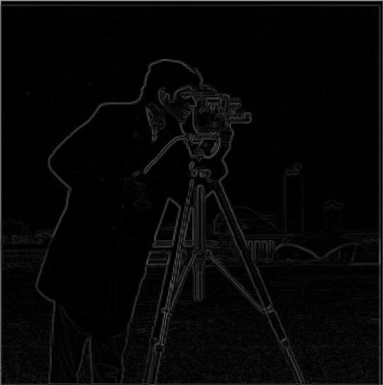
Note that the binarized result is far less noisy than before, although the lines are thicker.
We get the same results if we convolve the two convolution matrices together before applying to the cameraman.

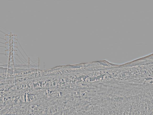
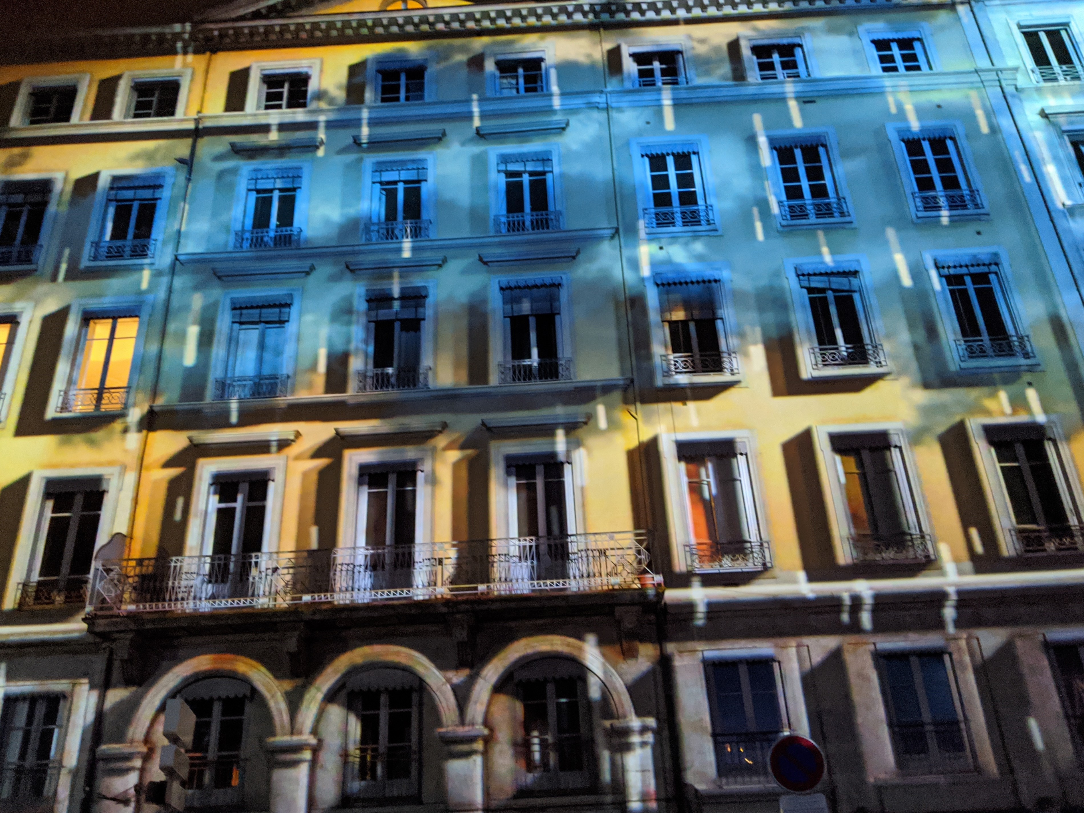
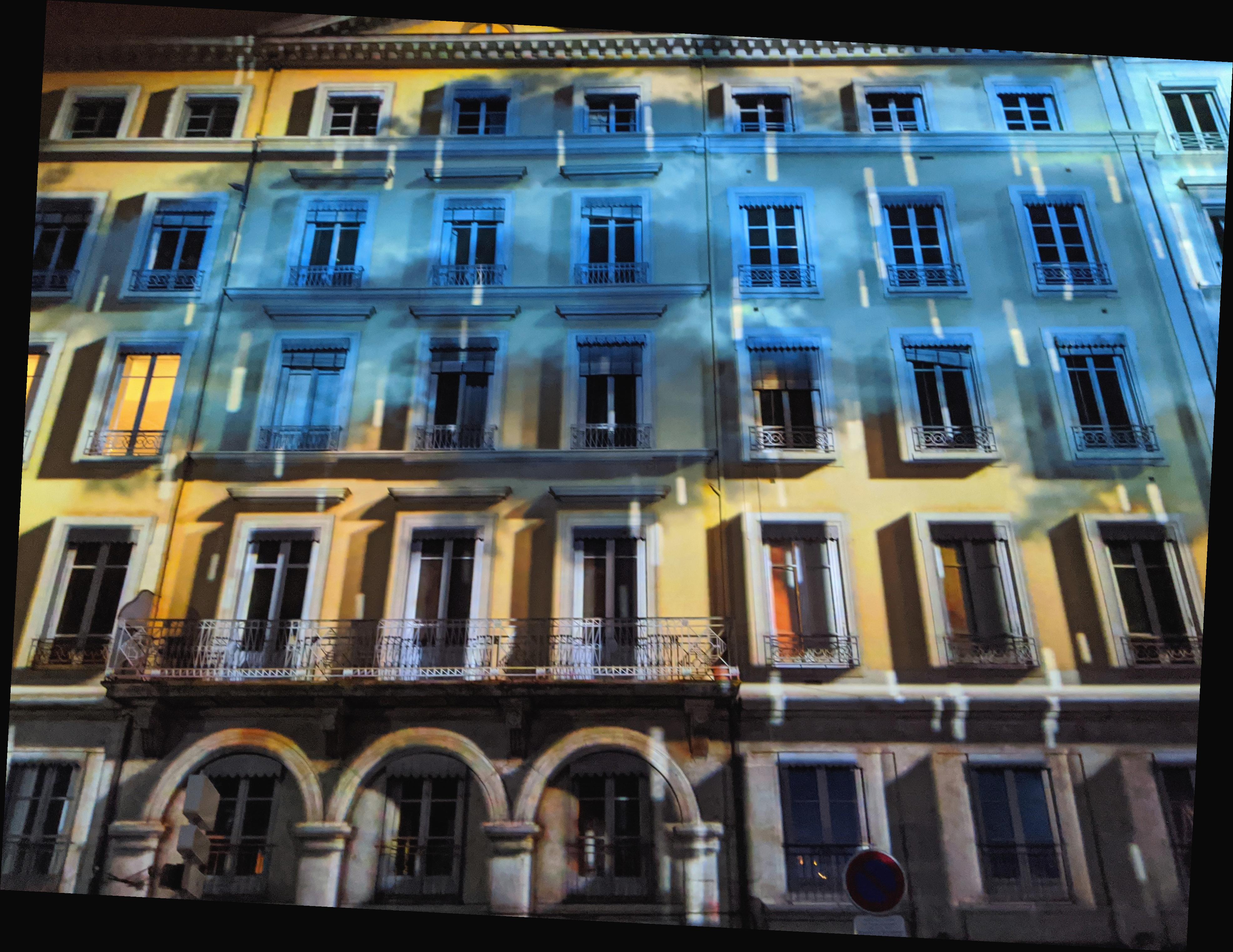
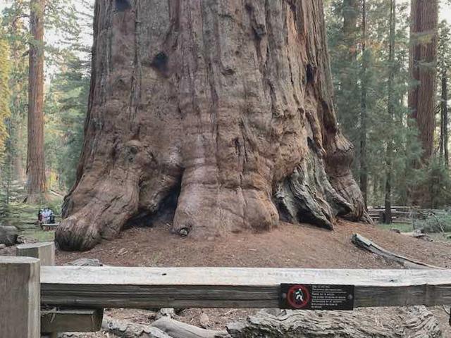
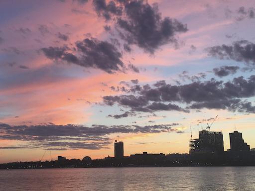
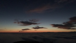
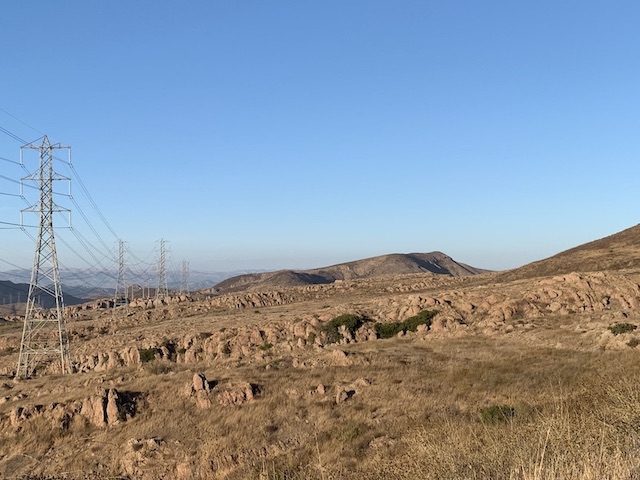
The original, unstraightened image we are working with:
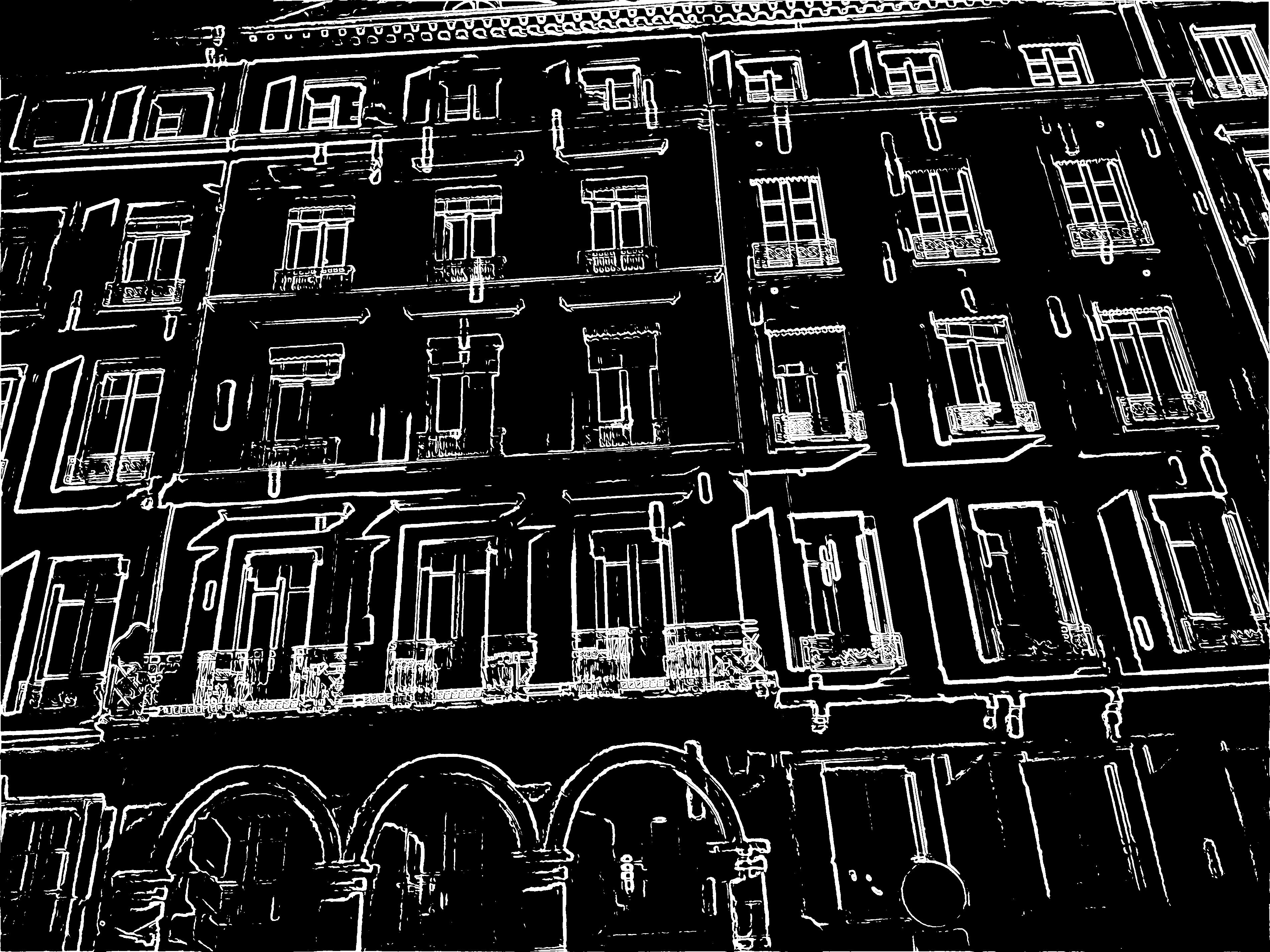
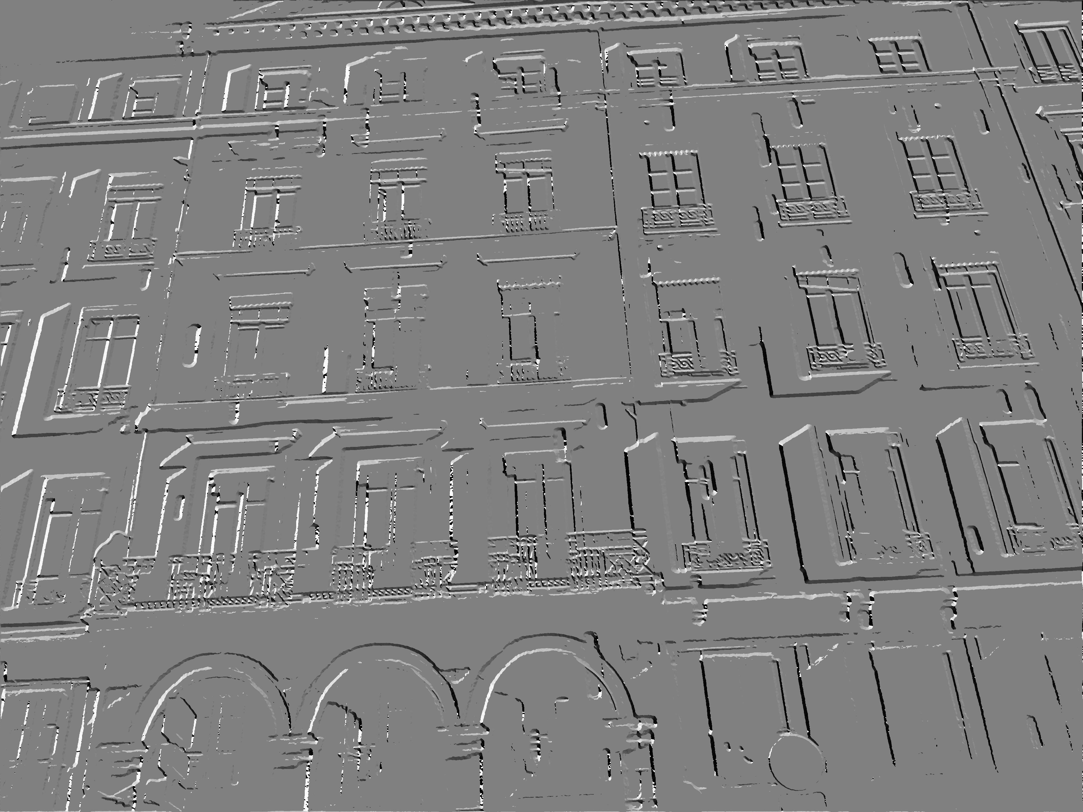
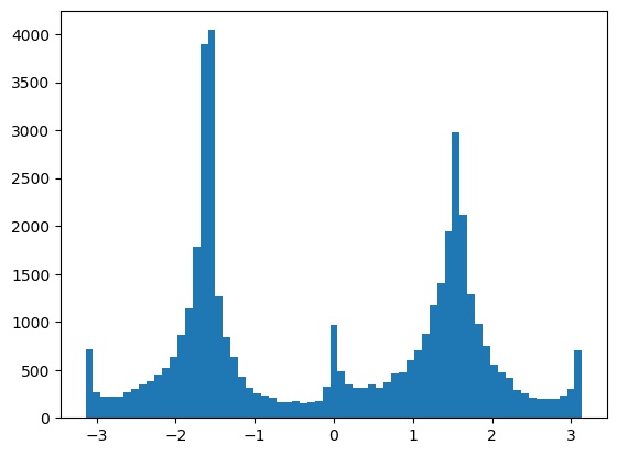
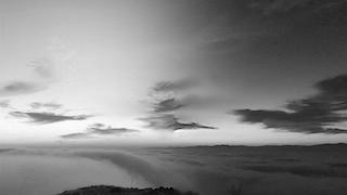
Using the same process as in 1.2, we get a binarized gradient magnitude image. In addition, we compute a binarized gradient orientation image, binarized on the same threshold as the gradient magnitude.
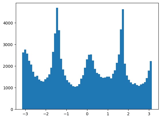
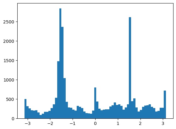
From this, we obtain a historgram of the gradient orientations in \((-\pi, \pi)\):
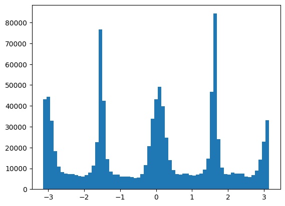
and we try rotations in the range \([-10, 10]\) to see which maximizes the size of the bins near \(0\), \(90\), \(180\), and \(270\) degrees.
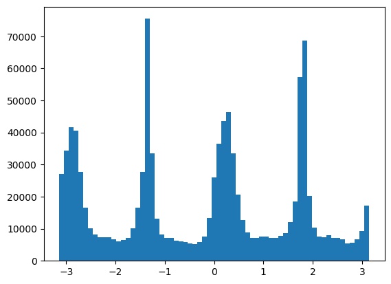
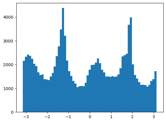
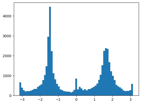
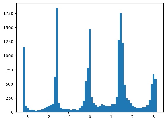
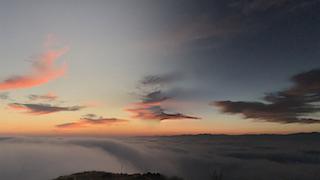
This results in the following best histogram and aligned image, with a -3 degree rotation:
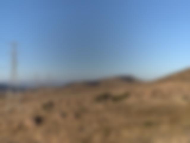
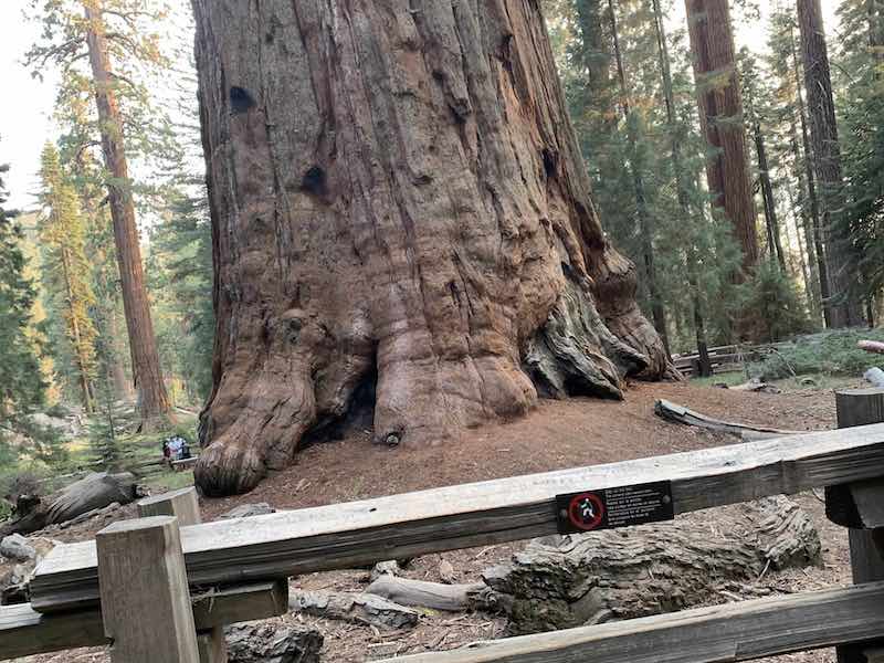
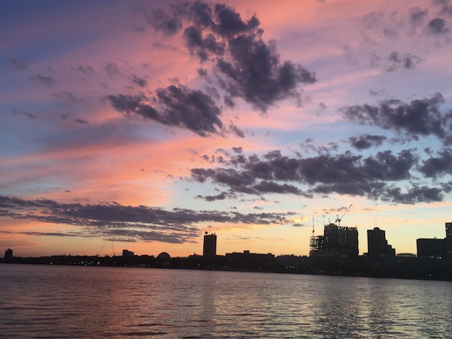
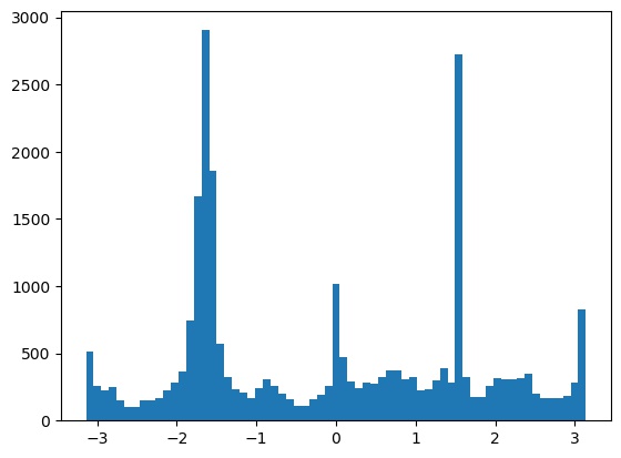
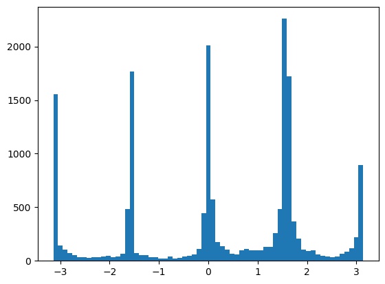
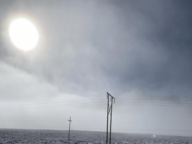
Alignment results on some other images. The result on the snow image was a bit off, likely because the plants and clouds confused the algorithm.


We can artificially sharpen an image by getting the image "details" as \(s(i) = i - G(i)\), where \(i\) is the original image and \(G\) applies a Gaussian smoothing filter. Then we add this sharpened image back in: \(i' = i + \alpha s(i)\) for some constant \(\alpha\).
Below, see the results on some images:


However, this does not actually add any new detail, it just tries to emphasize what detail is already there. Consider this blurred image, re-sharpened through the above process: it is not as crisp as the original.


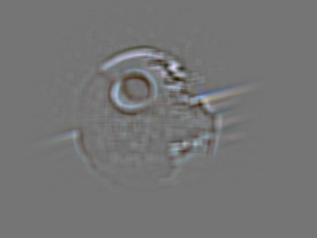
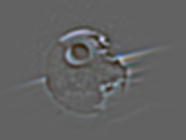
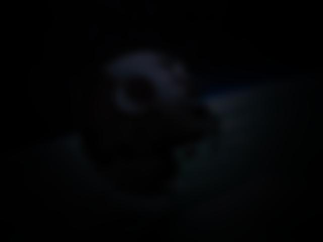
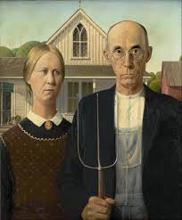
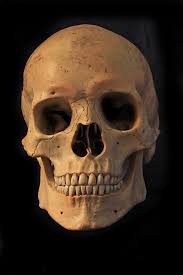
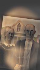
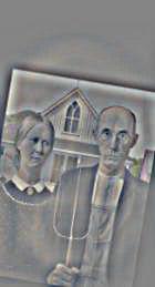
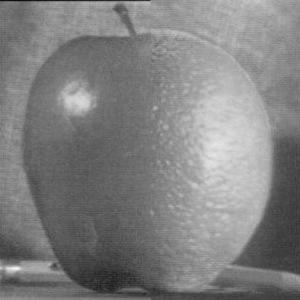
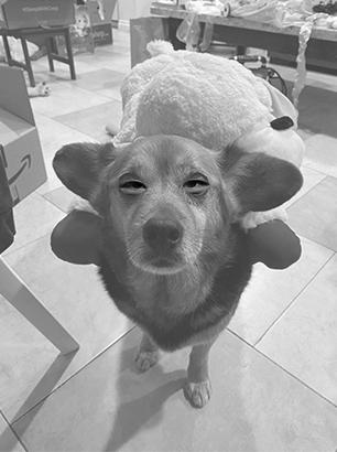
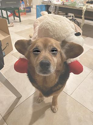
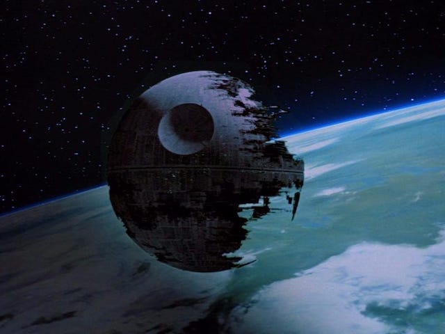
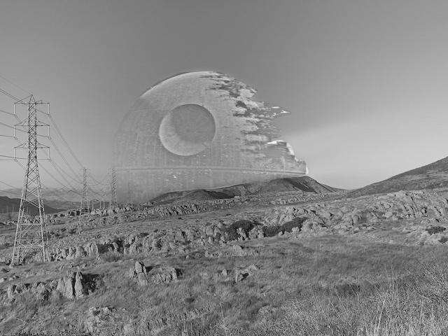
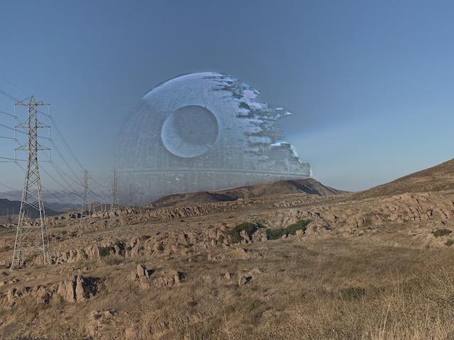
We combine the low frequencies of one image with the high frequencies of another to create hybrid images. Note that the first image is high-passed, and the second is low-passed.
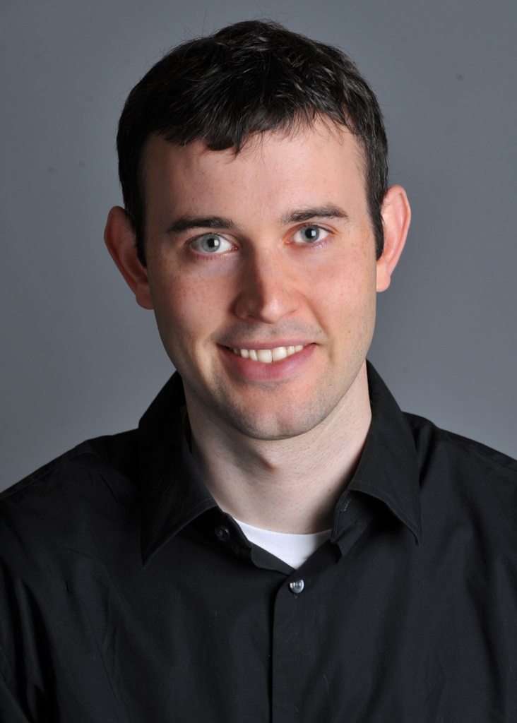
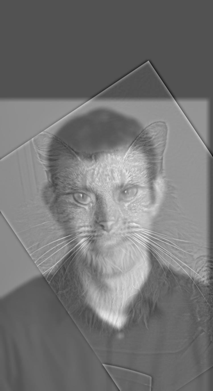
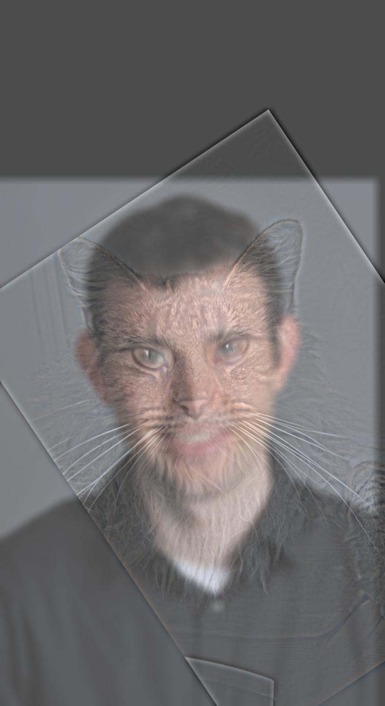
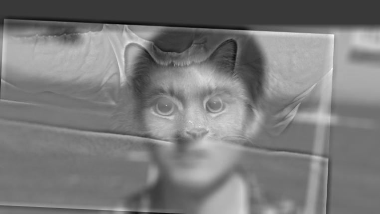
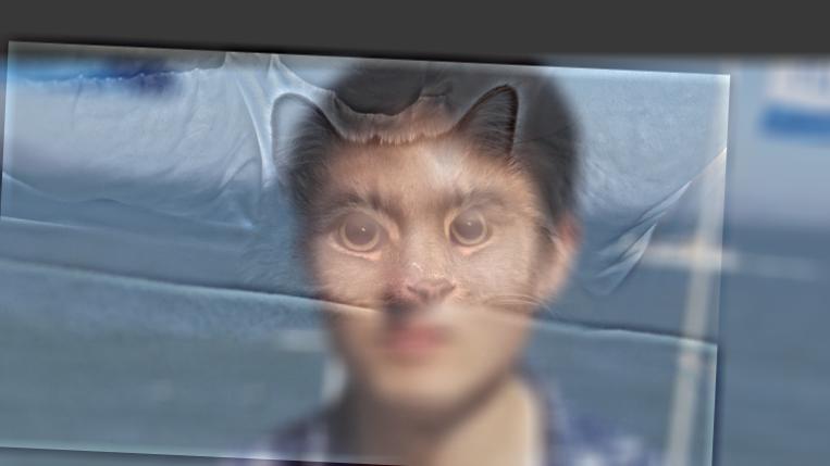
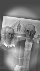
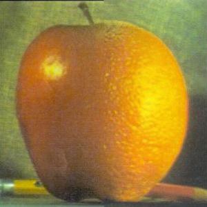
Interestingly, the colored results seem to mostly use the colors of the low frequency components. It seems the color information of a picture may often be low frequency.
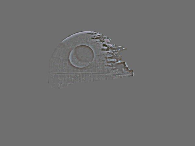
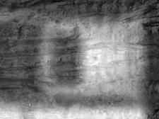
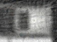
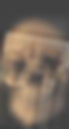
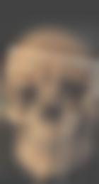
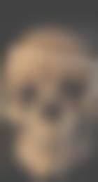
To get a closer look at what's going on, we can also look at the log magnitude of the Fourier transforms for the inputs, the filtered images, and the hybrid image. We will do this for the American Gothic and Skull images.
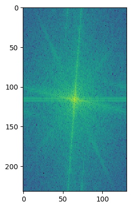
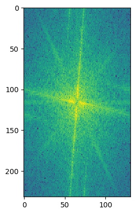
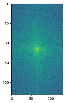
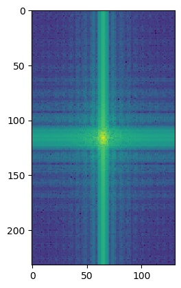
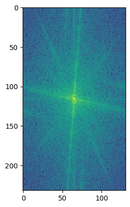
I'm not really sure what causes the grid lines in the low passed skull's Fourier's log magnitude graph.
We get Gaussian stacks by repeatedly passing the image through a Gaussian filter, and Laplacian stacks by finding the difference between consecutive Gaussian stacks.

Gaussian stack:


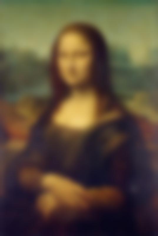
Laplacian stack:
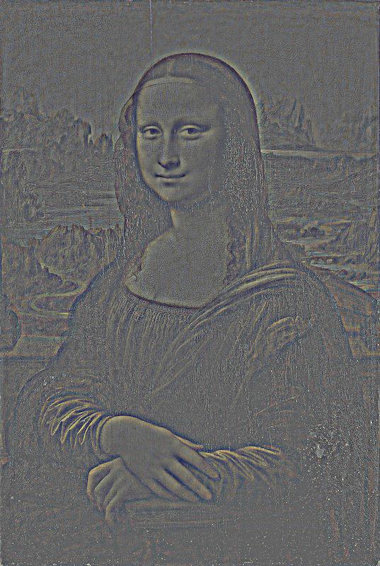
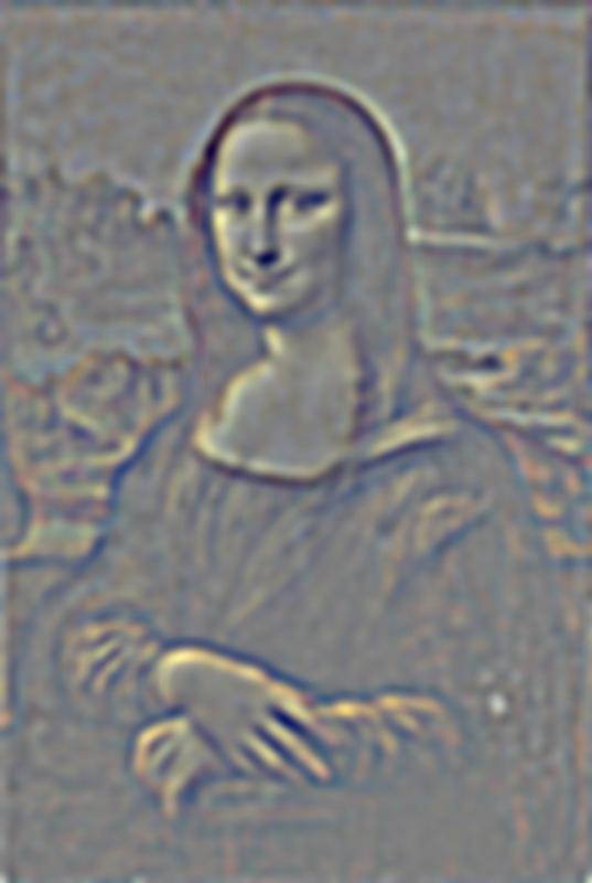
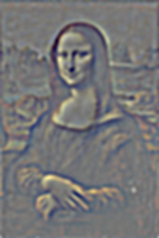
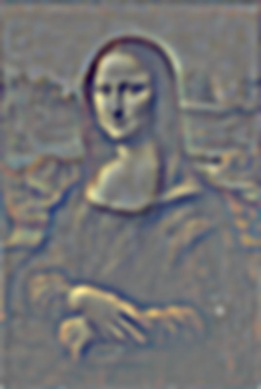
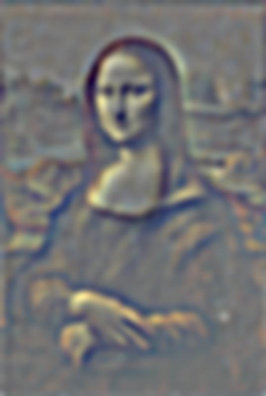
One thing we can notice on the Mona Lisa is that she is smiling at the first level of the Laplacian stack, but not the last.
We can also apply this procedure to one of the hybrid images from part 2.2:

Gaussian stack:


Laplacian stack:


In this way, we can roughly recover the original American Gothic and Skull images.
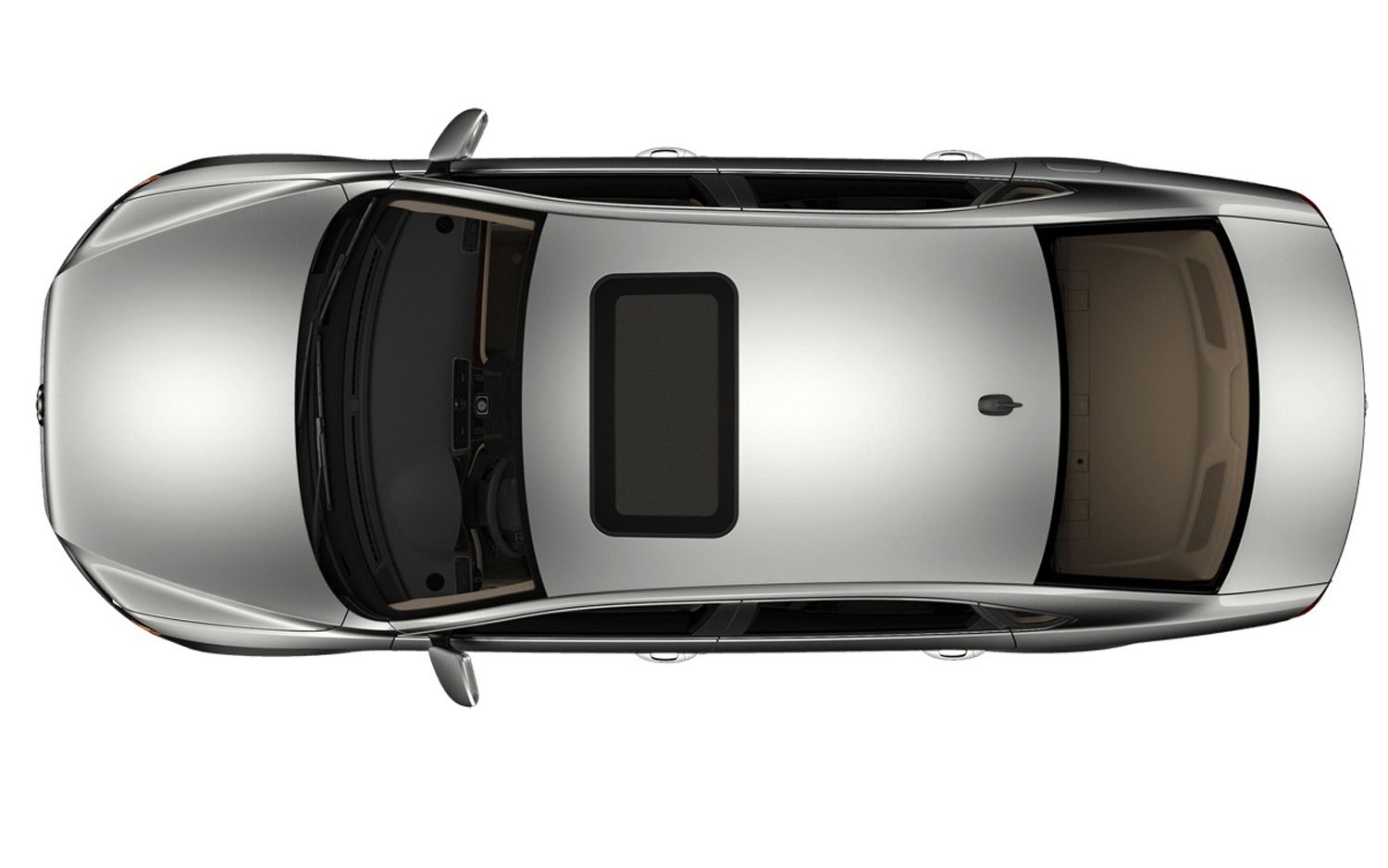
In this section, we blend images by blending their Laplacian layers (and the last Gaussian layer) with different levels of a Gaussian stack on a binary mask, such that higher frequency bands get a sharper mask and lower frequency bands get a blurrier one. Specifically, the equation at each level looks like $$L_c = G_m * L_a + (1 - G_m) * L_b$$ where \(L_a\), \(L_b\) are the Laplacian levels of the original images; \(G_m\) is the Gaussian level of the mask; and \(L_c\) is the Laplacian level of the result.
Below are some results using a binary left/right mask:


The next results use an irregular mask.


Finally, here are the masks as applied to various levels of the two images in the last blended image: