Overview
This project was an exercise in filtering, blurring, blending, and aligning images. The centerpiece of all these operations is the Gaussian filter, which is implemented in part 1.
lead up to the Gaussian: part 1.1
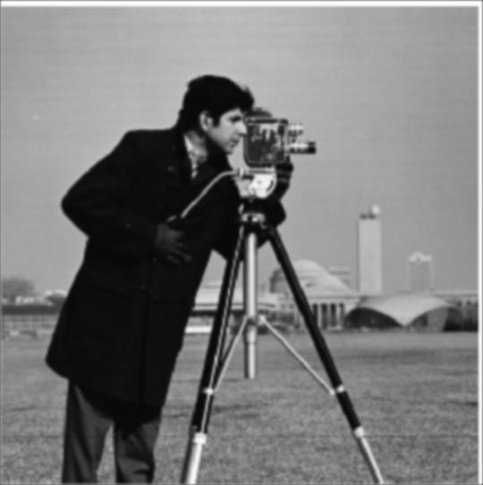
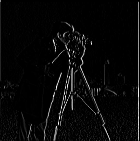
Starting with a finite difference operator and this cameraman, let's do some filtering:
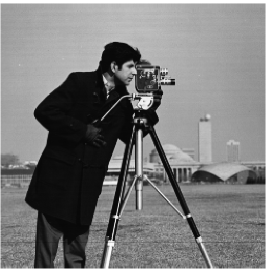 original for reference's sake
|
 convolution with finite difference of dx
|
 convolution with finite difference of dy
|
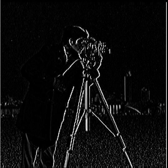
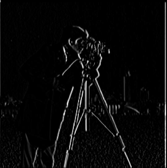
 edges before binarizing gradient
|
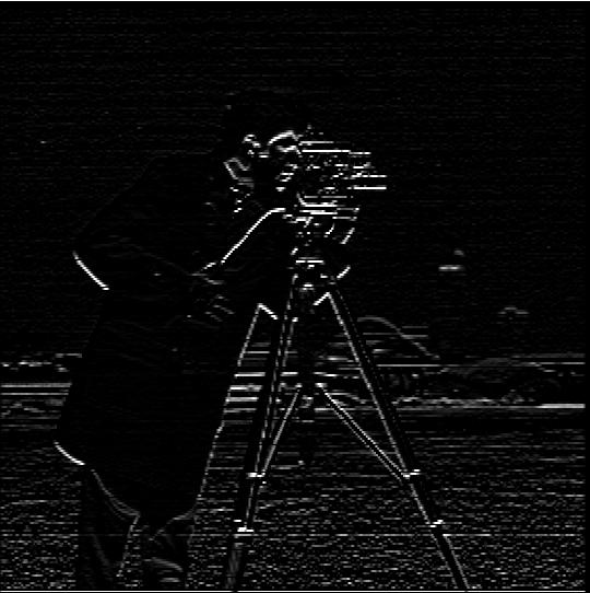
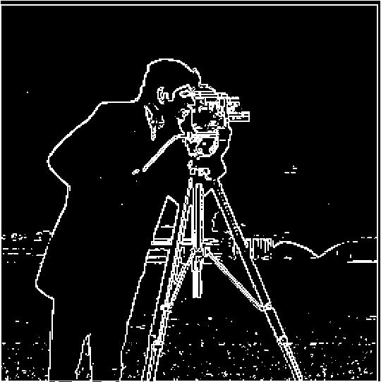 threshold: magnitudes > .5
|
Even with just this, we get a sense of where the edges are. But it's very noisy, and a lot of detail gets lost when trying to binarize magnitudes above/below a certain threshold. So let's see what Gaussian filters can do about that...
1.2 The DoG filter
 original with Gaussian
|
 original image convolved with dx -> dx image -> convolved with Gaussian
|
 original image convolved with dx -> dx image -> convolved with Gaussian
|
The nice thing about convolutions is that they're associative, which means a derivative of the Gaussian filter
can be precomputed so it doesn't have to convolve with every image twice. This means you can get the same results as above with just one convolution of the original image instead of two.
Here are the original images convolved with the derivative of the Gaussian:
 Gaussian convolved with Dx -> DoGx operator -> convolve with original image
|
 Gaussian convolved with Dy -> DoGy operator -> convolve with original image
|
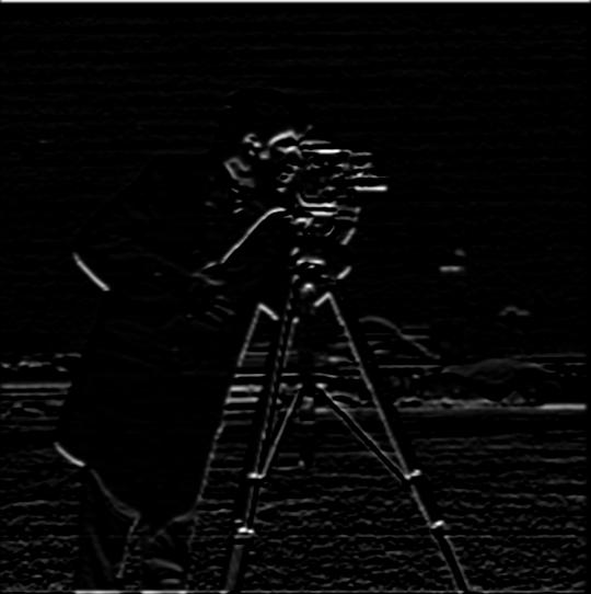
For completeness's sake, here are the edges after being convolved with the derivative of Gaussian filter:
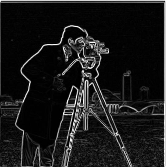 edges with Gaussian
|
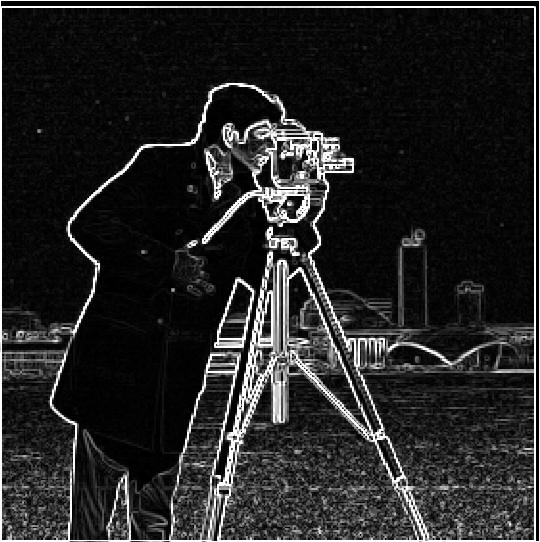
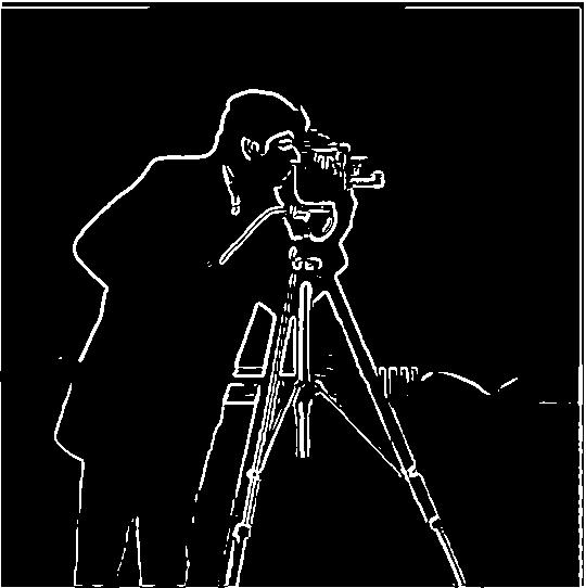 binarized with threshold >.5
|
The binarized Gaussian edge image looks amazing (to me). I know a lot of information is lost the higher I make the magnitude threshold, but the denoising of the gaussian filter and high threshold produces such nice, crisp, bold edges that I can't resist it!
The computation of the gradient magnitude was to square all dx terms and square all dy terms, then sum them together and take the square root of that. The resulting array is now on the range [0, 1]
where high values indicate a large change and low values indicate little change. The gradient points in the direction of the most rapid change and the magnitude is the 'intensity' of that change.
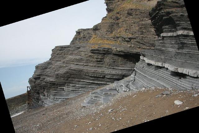
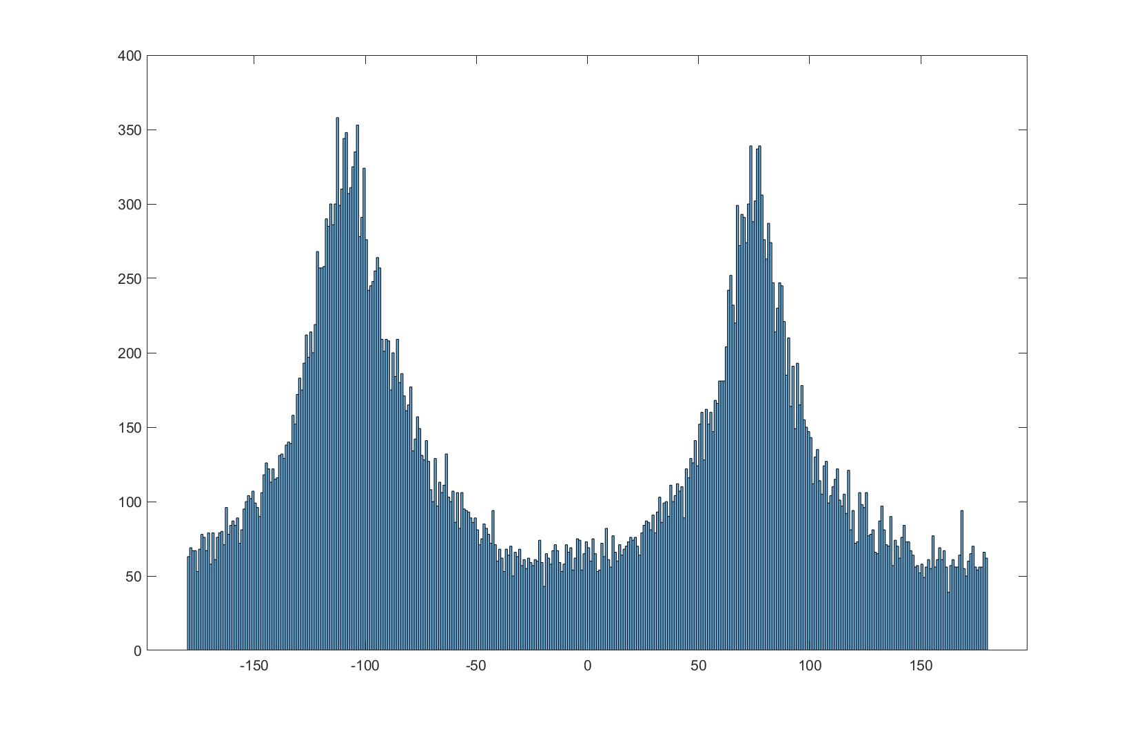
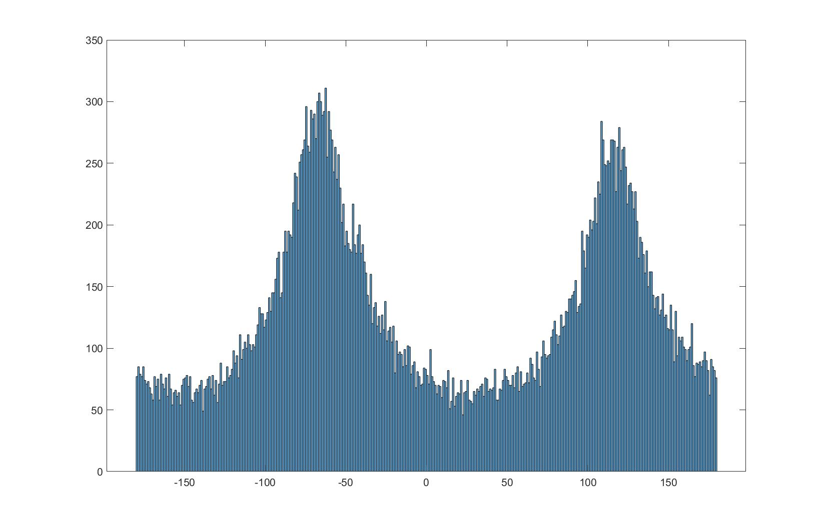
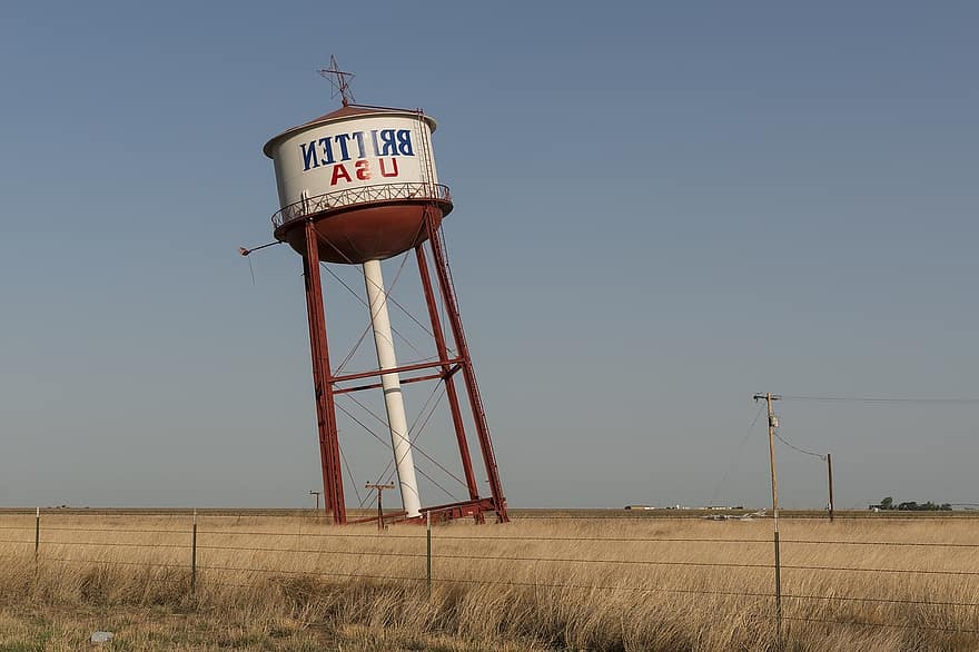
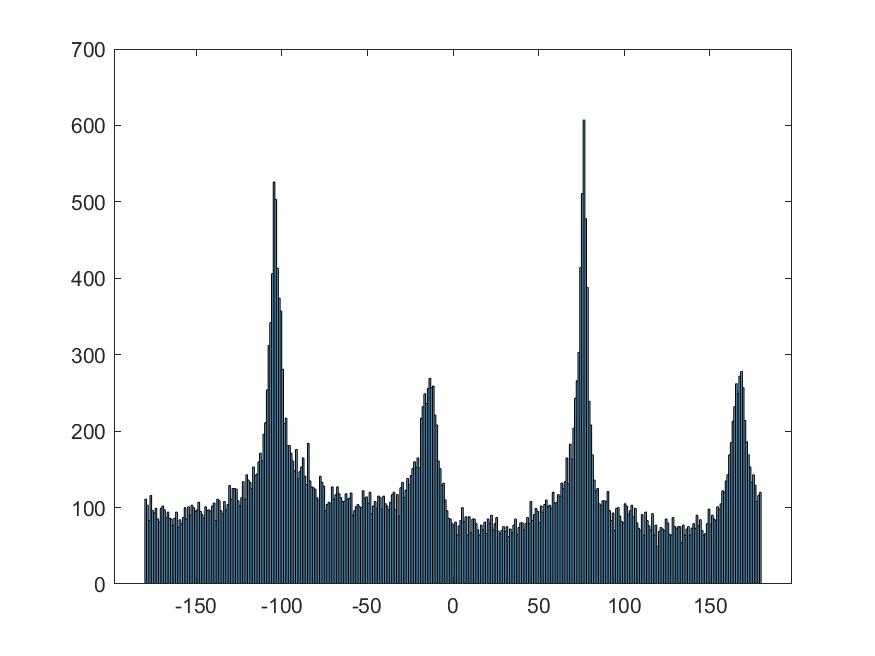
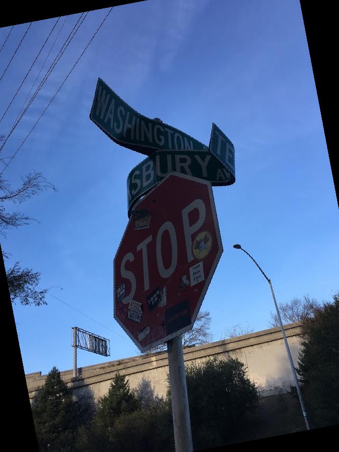
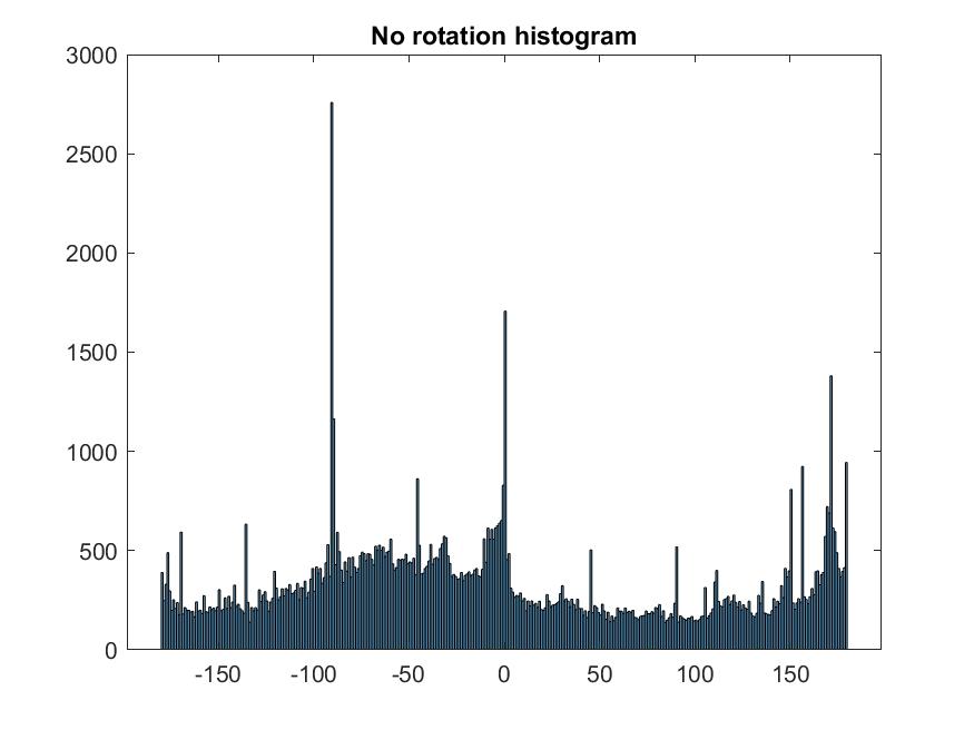
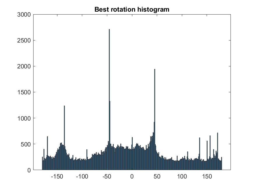
1.3 Image straightening
Using the angle of the gradients at edges above a certain threshold, we can 'score' images based on their number of horizontal/vertical edges to straighten something that's crooked.
I initially used a [-180, 180] degree window, but too many images ended up flipping upside down or to the left/right, so I narrowed the window to [-45, 45] and got much better results.
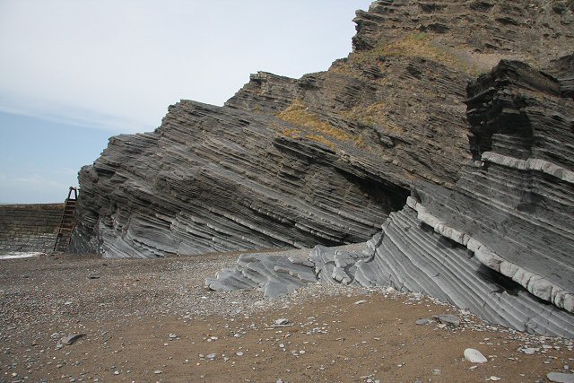
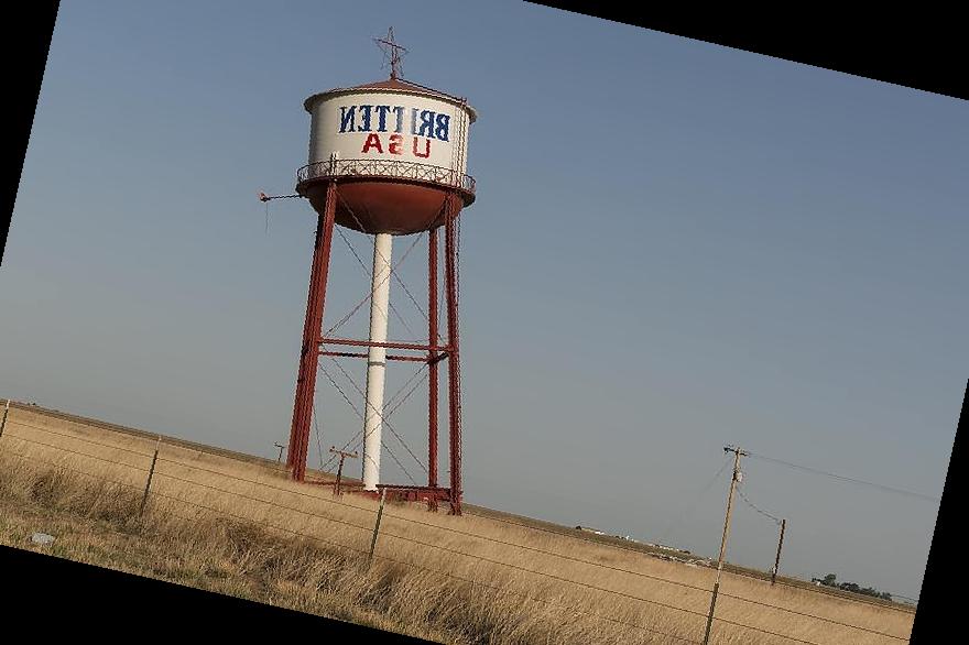
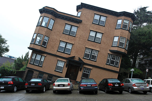
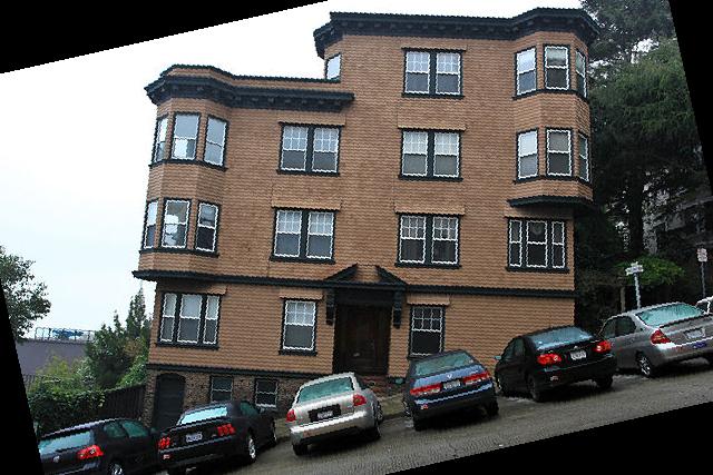
 tilted
|
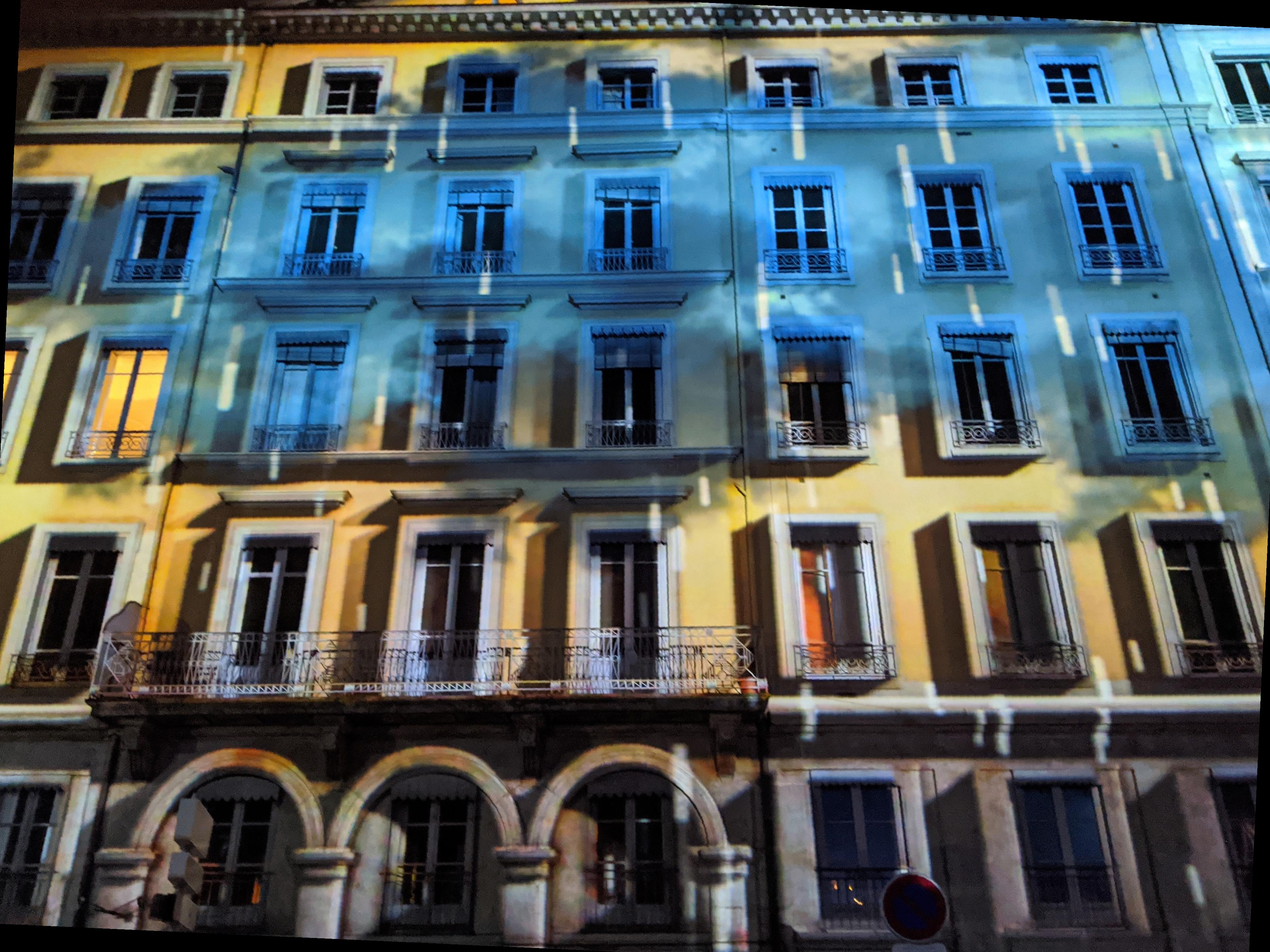 best angle: -2.586206896551724 degrees
|
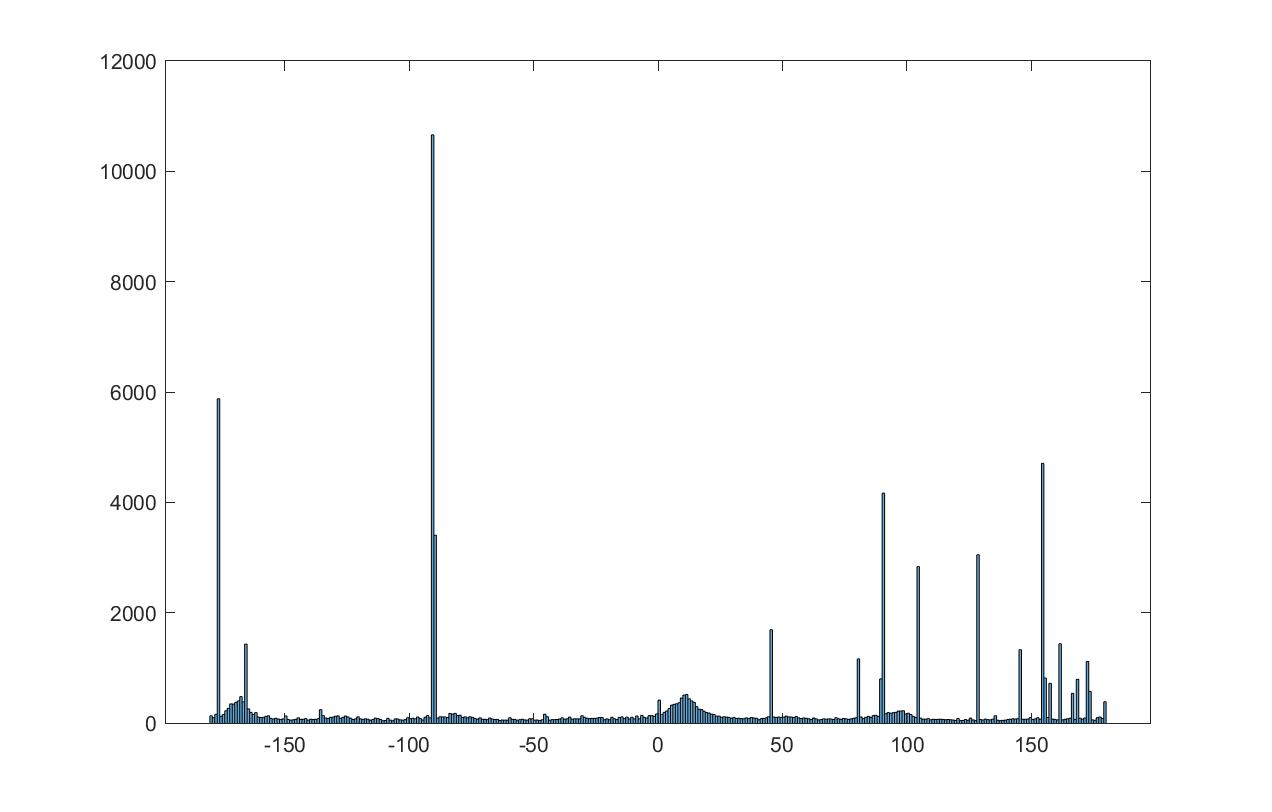
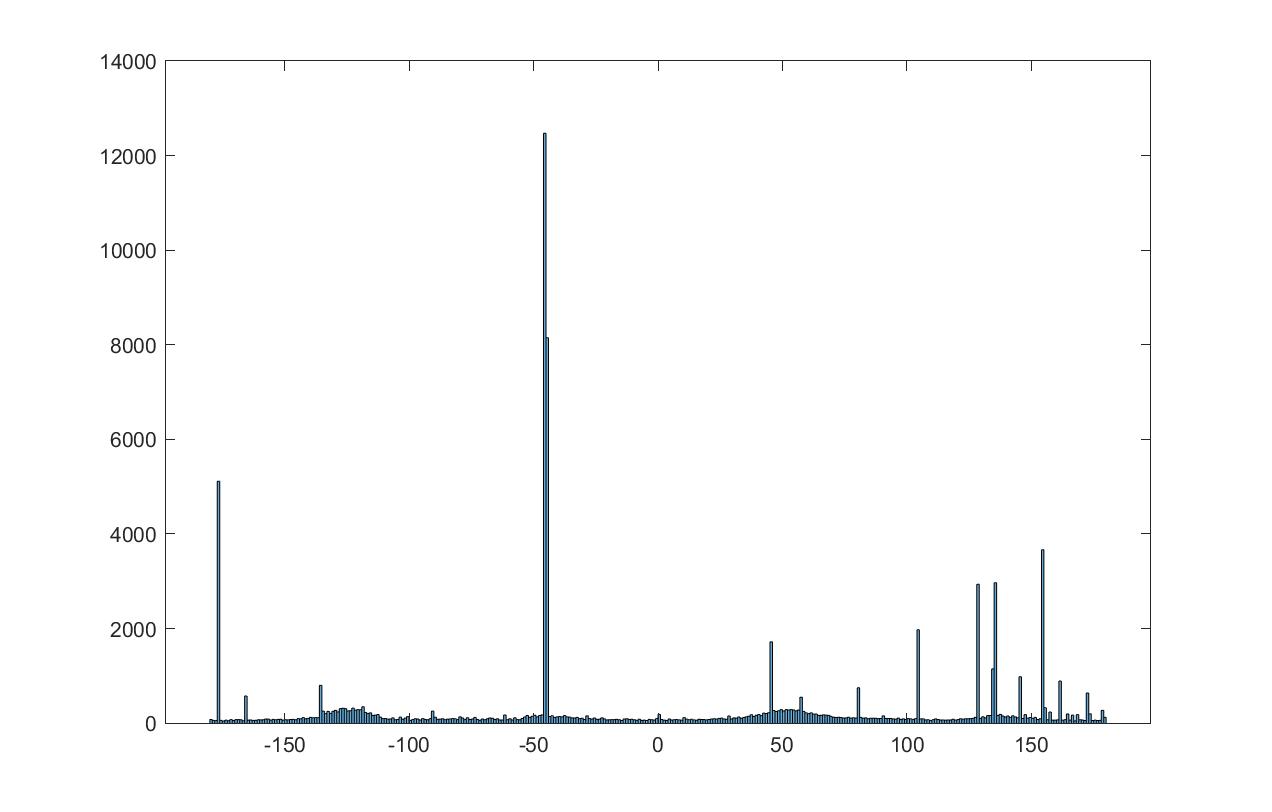
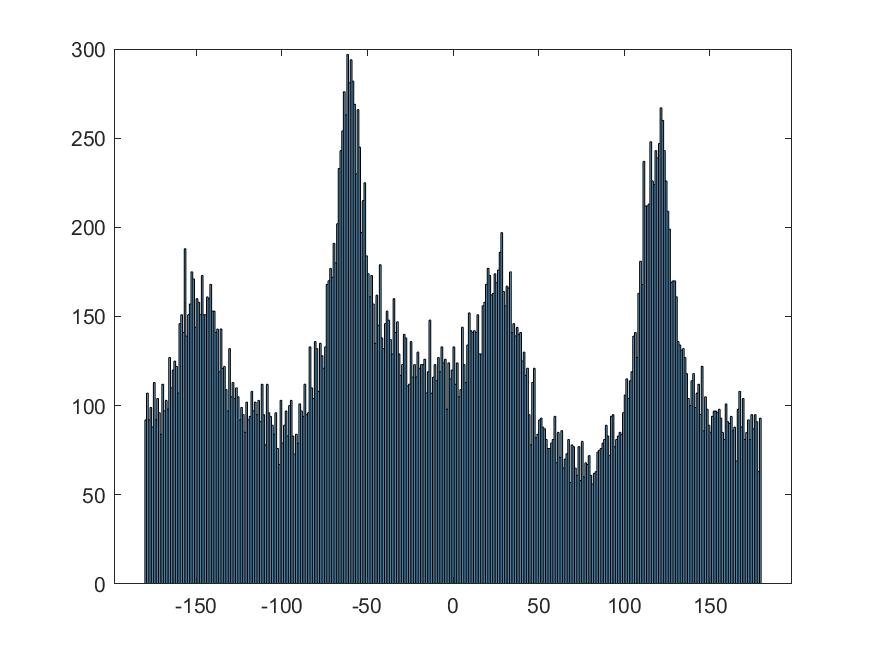
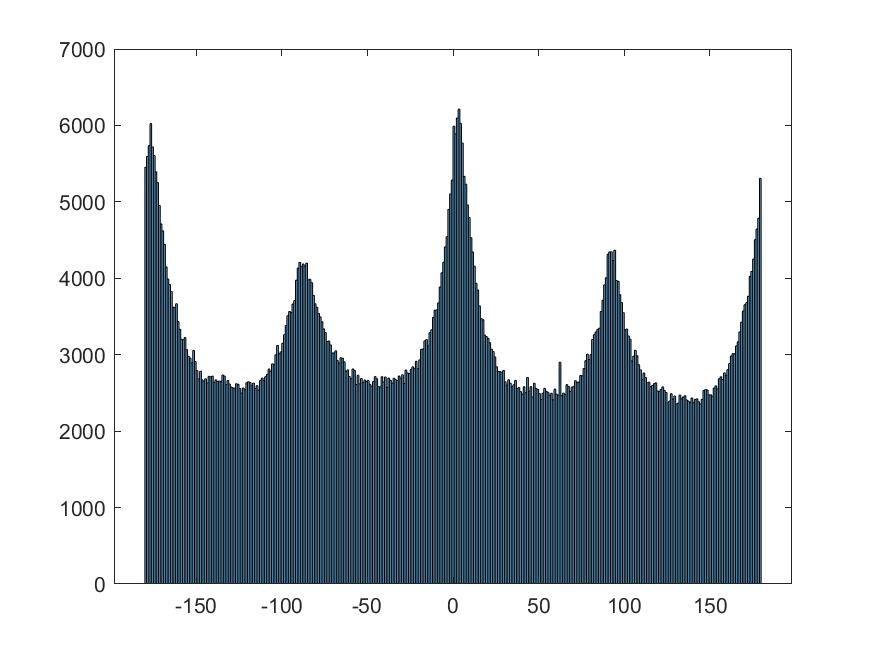 no rotation histogram
|
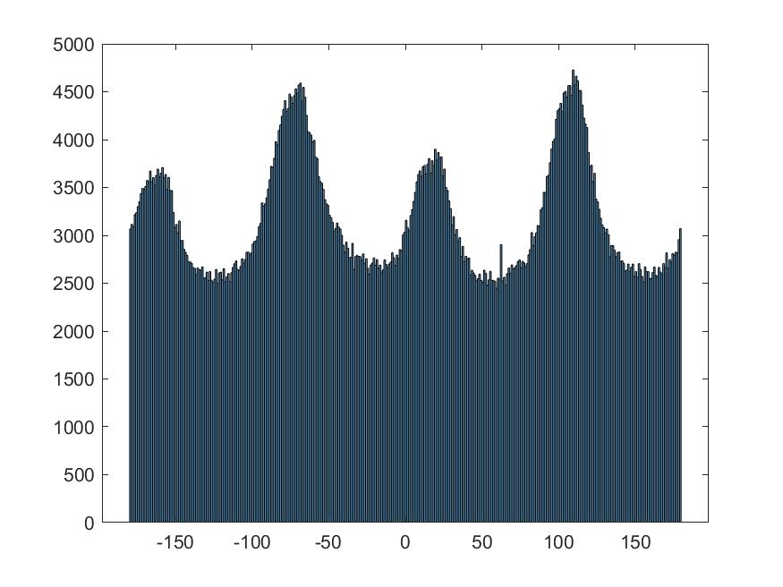 best rotation histogram-- note the increase in angles at -180 -90, 0, 90, 180
|
 tilted
|
 best angle: 16.685393258426966 degrees
|
 no rotation histogram
|
 best rotation histogram
|
|
 best angle: -12.640449438202248 degrees
|
 no rotation histogram
|
 "best" rotation histogram
|
 'tilted'
|
 best angle: 12.640449438202248 degrees
|
 no rotation histogram
|
 best rotation histogram
|
failed case:
 I think the horizon/edges were too powerful to move this one very much....
|
 'best' angle: 10.617977528089888 degrees
|
 no rotation histogram
|
 best rotation histogram
|
Fun with frequencies
2.1- Image "sharpening"
 original
|
 unsharp filter
|
Here are some of my own images:
 original
|
 unsharpened
|
 original
|
 unsharpened
|
Now, for a sharp->blurred->unsharpened image:
 original
|
 blurred
|
 unsharpened - some detail couldn't be restored, but it's better than blurred
|
2.2- Hybrid images
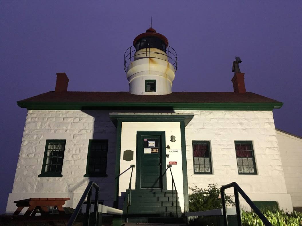 a lighthouse...
|
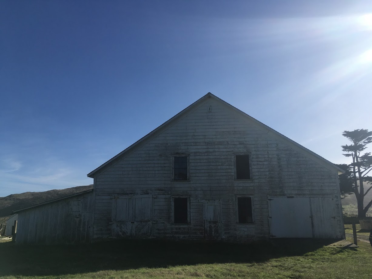 and a house....
|
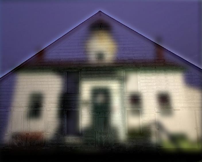 make a houselight!
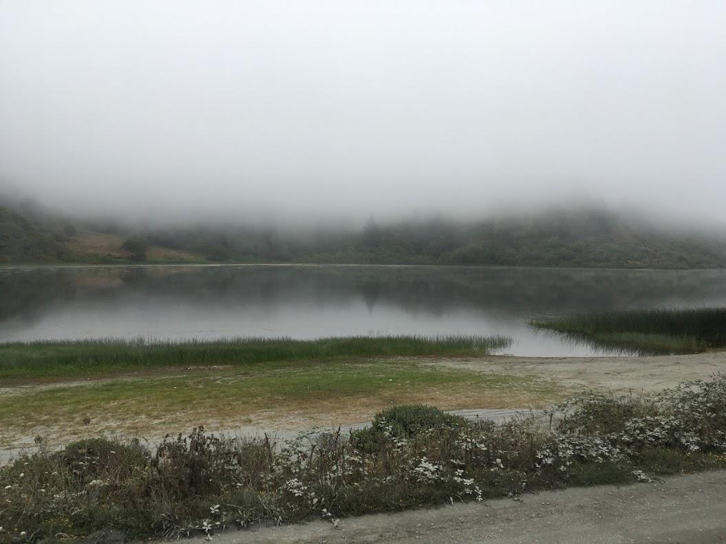
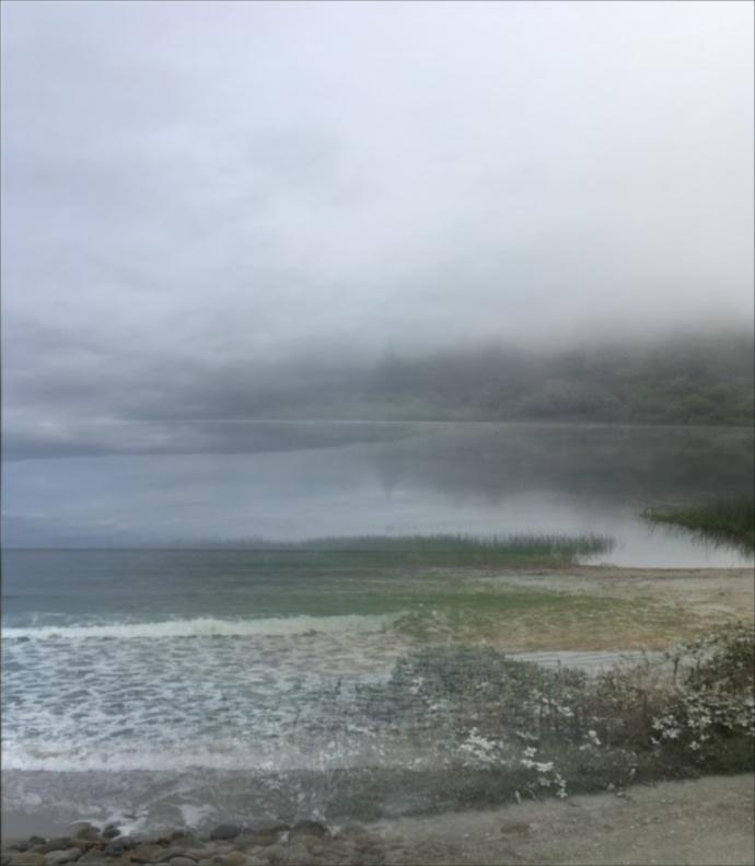
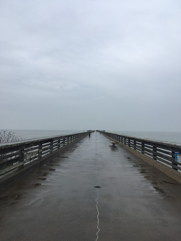 a pier
|
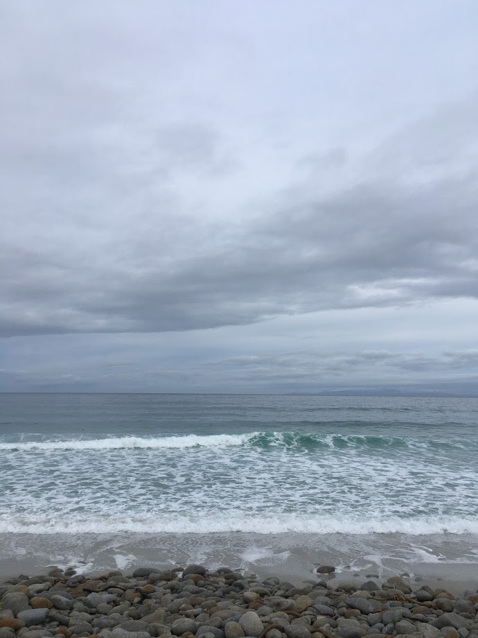
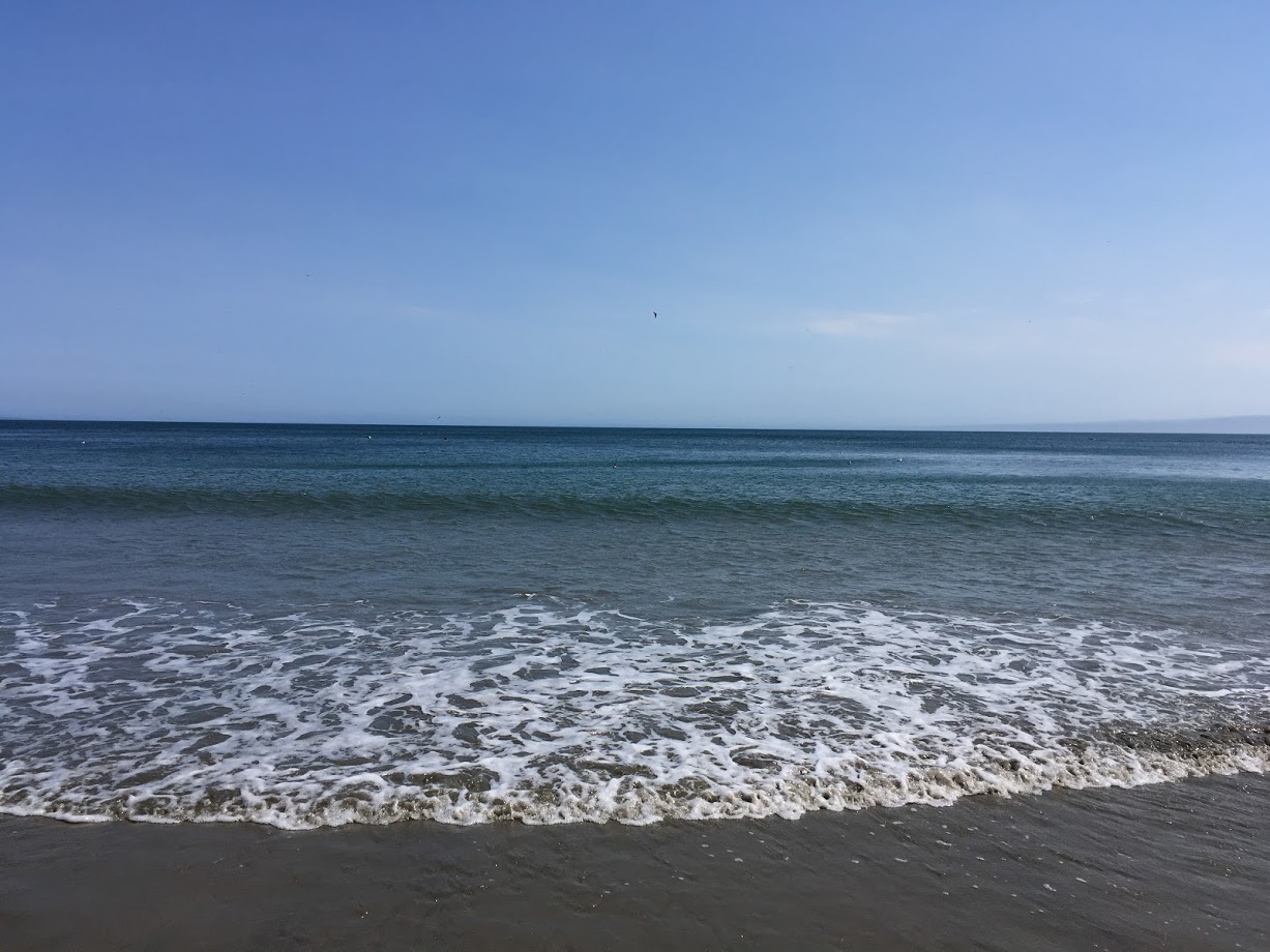 a beach
|
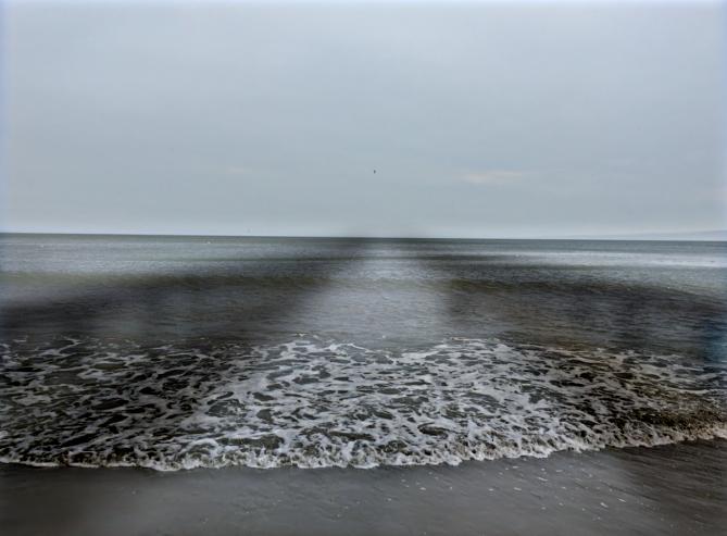 make a pierbeach
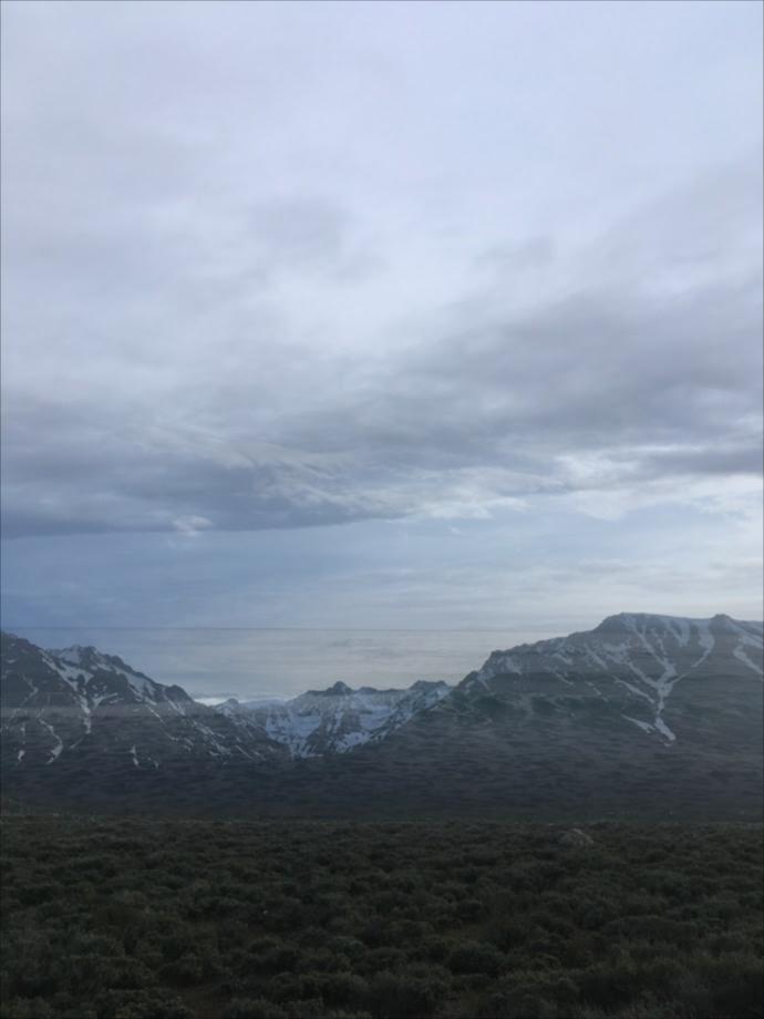
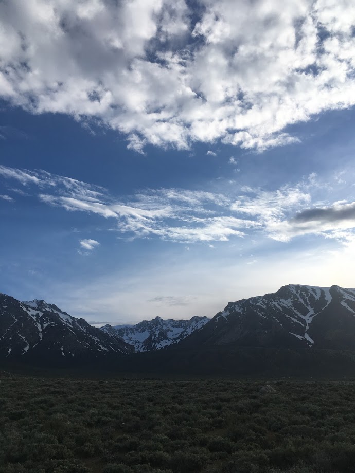 Mountains....
|
 and the beach....
|
 make an oceantain!
Favorite result with frequency domain:
 the low frequency image
|
the high frequency image
|
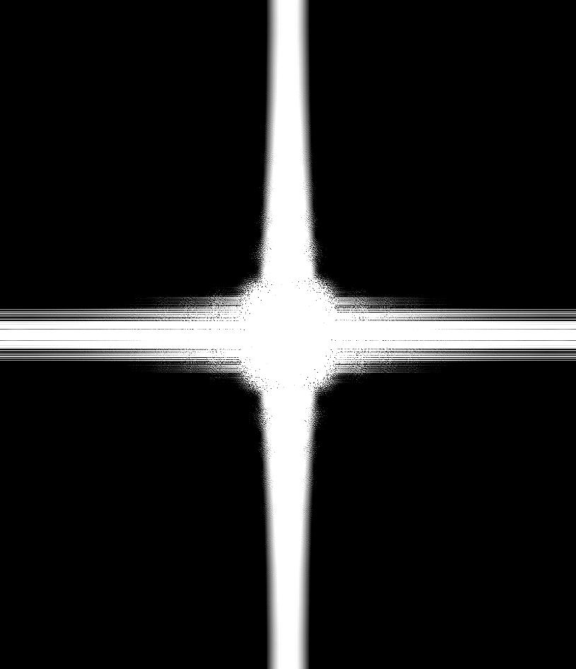
 fourier transform of the image before any aligning/etc
|
 fourier transform of the image before any aligning/etc
|
 filter applied
|
 filter applied
|
 hybrid
|
 fft of hybrid
|
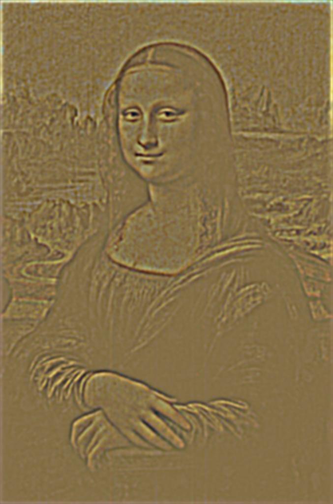
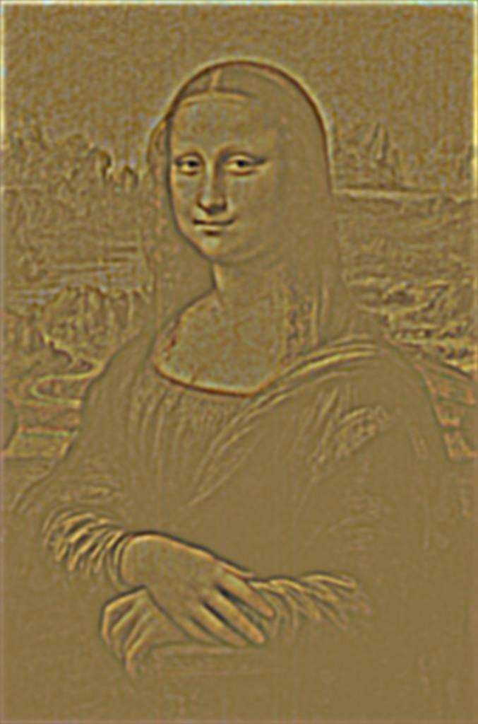
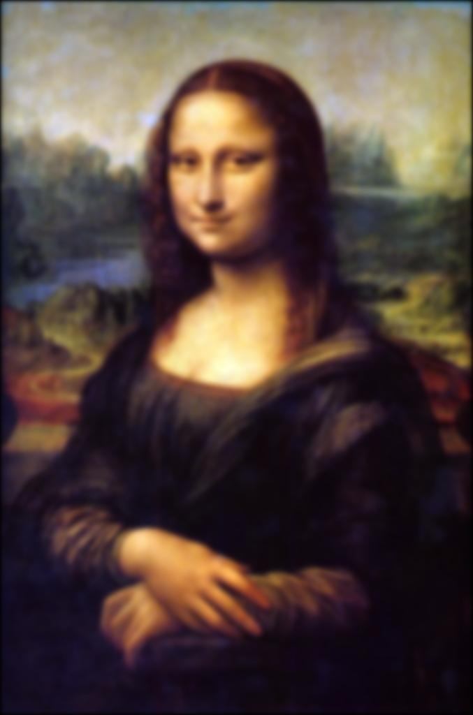
Part 2.3 - fun with stacks
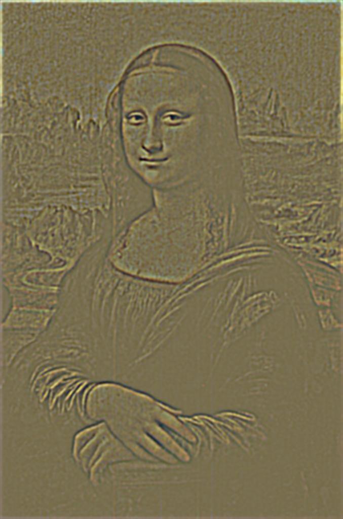
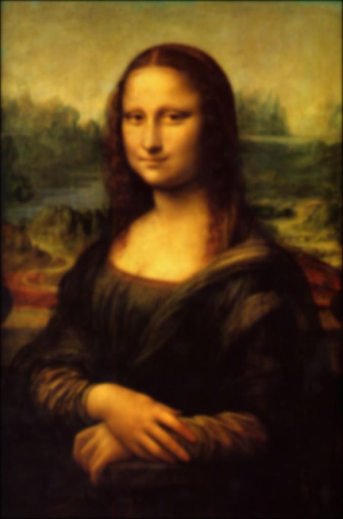
One fun thing about breaking an image into its low and high frequency portions is that we can see different 'expressions'
of an image, like the Mona Lisa. I don't know if this is because I can't really step back from my desk (I'm up against a corner wall in my room),
but I don't really see the smile/frown or the shift in her eyes. She always looks like she's smirking while looking at the viewer to me.
 Gaussian level 1
|
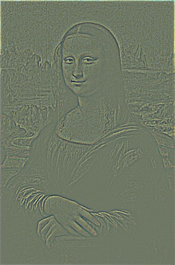 Laplacian level 1
|
 Gaussian level 2
|
 Laplacian level 2
|
 Gaussian level 3
|
 Laplacian level 3
|
 Gaussian level 4
|
 Laplacian level 4
|
 Gaussian level 5
|
 Laplacian level 5
|
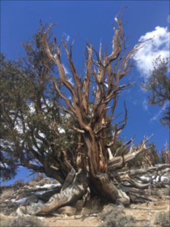
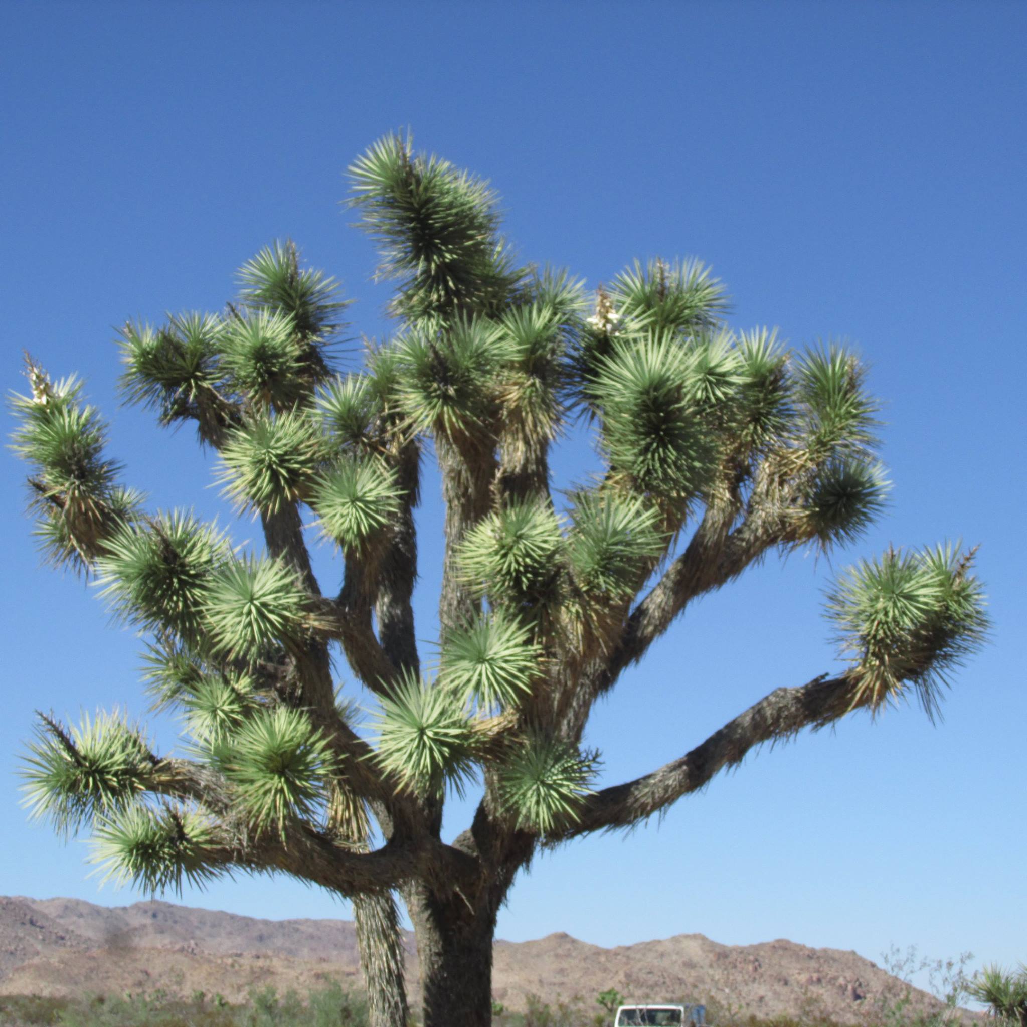
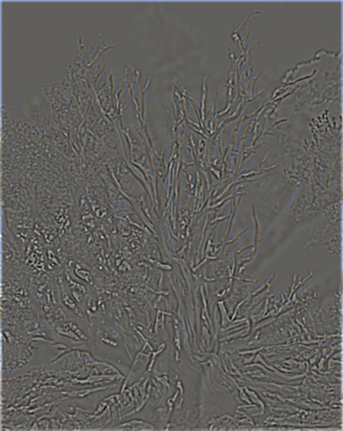
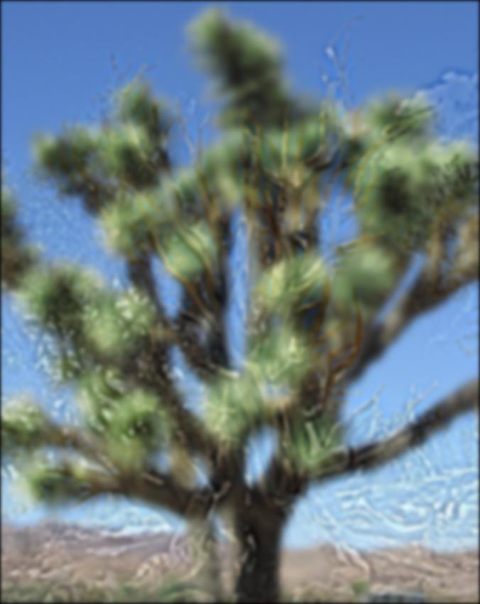
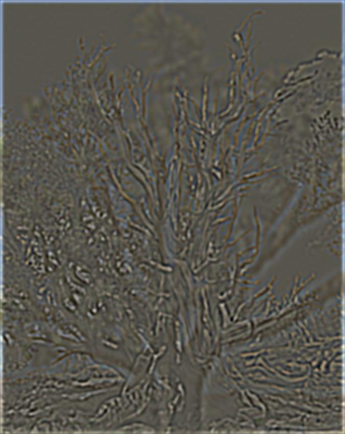
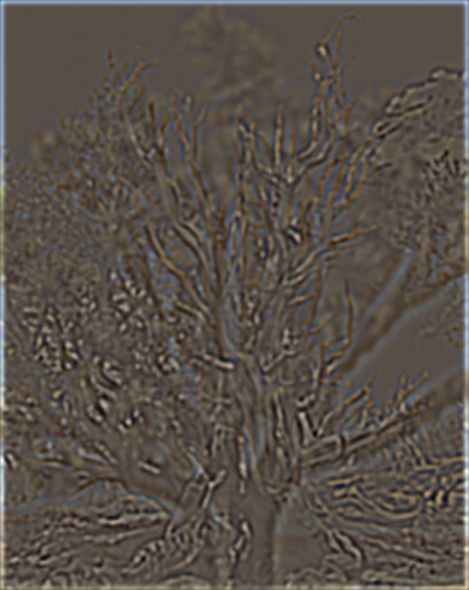
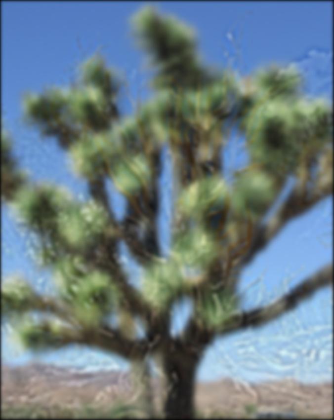
And now, a return the Methuselah/cholla trees from earlier. These images were 'unhybridized' by using the same
Gaussian and Laplacian stacks that revealed the Mona Lisa's hidden low frequency and high frequency 'subimages'. In this case,
I know that the cholla tree was low frequency and the methuselah tree was the high frequency portion, so the fact that I can see a little bit more of
each respective tree in their stack isn't too surprising, but what does surprise me is how embedded they are and difficult to reverse once they've been
hybridized. I wonder if it's because I used sigma = 10 (to act as the cutoff frequency) for my hybrid images that I did for the Gaussian stacks (a 'normal' sigma of 1).
 Gaussian level 1
|
 Laplacian level 1
|
 Gaussian level 2
|
 Laplacian level 2
|
 Gaussian level 3
|
 Laplacian level 3
|
 Gaussian level 4
|
 Laplacian level 4
|
 Gaussian level 5
|
 Laplacian level 5
|
Part 2.4 Multiresolution blending
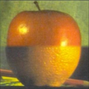
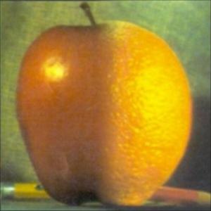
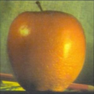
I think I may have gotten a bit lost on this step. I implemented my laplacian stacks, the mask, and used linear interpolation to 'seam' them together, but I found that
I got very different results from the website if I followed the paper's example and very different results from the paper if I tried to imitate the website's orapple.
Personally, I like the fully blended orapple on the website and I think the paper's orapple has too severe of a seam, even though I get what they're
trying to demonstrate with the example. I wanted to have the user select the blending region and I found that if I chose a very narrow region to be the mask, I would get
a clean, but abrupt seam like the paper and if I chose a large mask I would get a much more gradual blend like on the website.
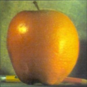
The orapple:
 ^a narrow horizontal mask around the midpoint of the apple
|
 ^a narrow vertical mask just to the right of the apple stem
|
 ^a broad vertical mask from the top-bottom of apple
|
 ^a broad horizontal mask just to the right of the apple stem to the rightmost edge of it
|
One other 'square' blend:
|
a beach...
|
 and a lake...
|
 make a beach lake!
For irregular masking, I'm not sure if I actually implemented it the way the paper did. I know the mask is no longer supposed to be a broad sweep of 1s and 0s from the
right/left or top/bottom of an image. I was able to implement an irregularly shaped mask and I used the same spline/stacks/summing/etc method as I did with the orapple, but
this is where the paper's method and mine differ.
What I had in mind was for a user to select an area in the image to blend using a freehand tool in matlab. Then, I would plot the centroid of that ROI on the 'base image ' that they would like to blend to,
and using that centroid as a reference point, select a new centroid for the thing to blend. I would mask it, circshift it, then use the Gaussian/Laplacian/spling stacks as before to blend it all together at various resolutions.
In the paper, I saw references to having one image be a 16x16 block, and pad it to get some overlap, then crop to the mask and blend it in to the other image, but I couldn't find a way to get that to work
with what I had in mind for the user. However, I think what I was able to produce still accomplishes the task of multiresolution blending, but not quite in the way outlined by Burt and Adelson.
Irregular mask blends
|
a beach at Point Reyes...
|
a pier in Crescent City...
|
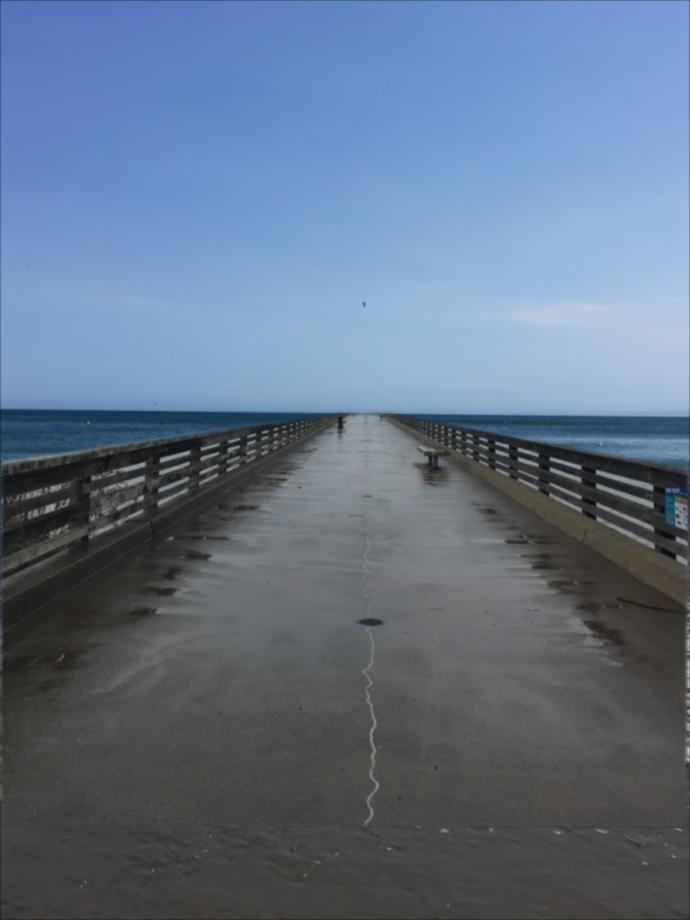 to make the Crescent Reyes pier
|
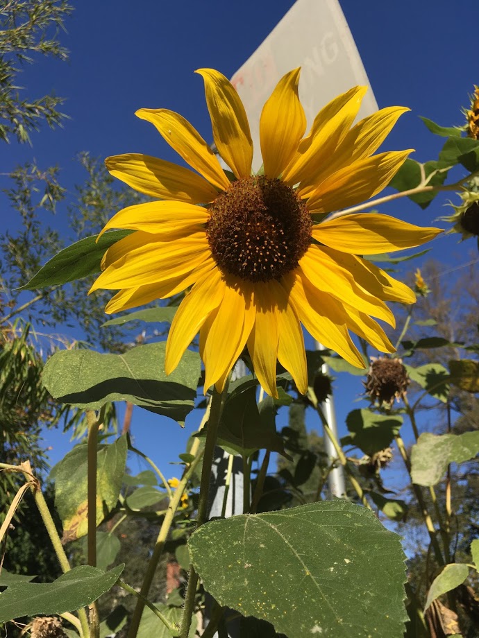 a sunflower...
|
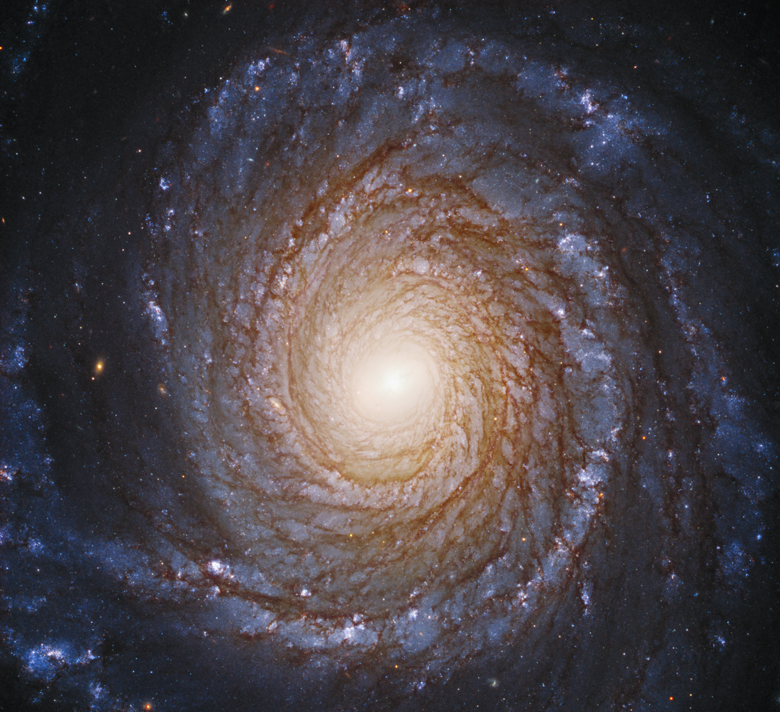 with the milky way galaxy...
|
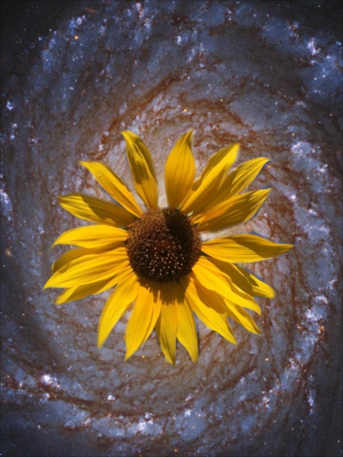 sunflower galaxy
|
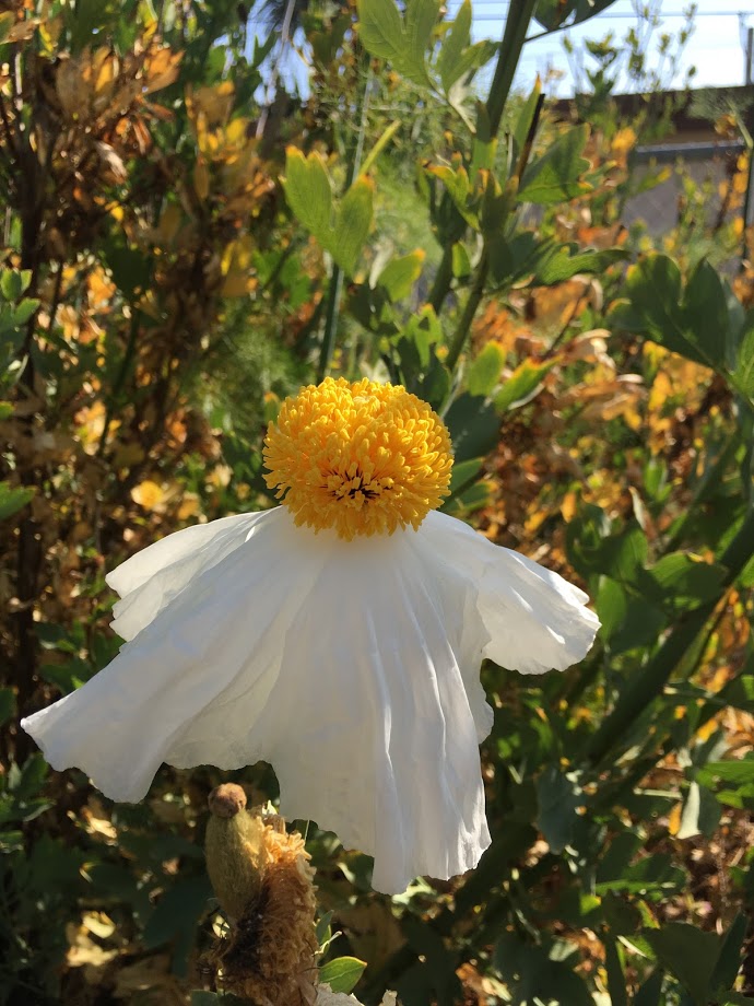 an eggflower...
|
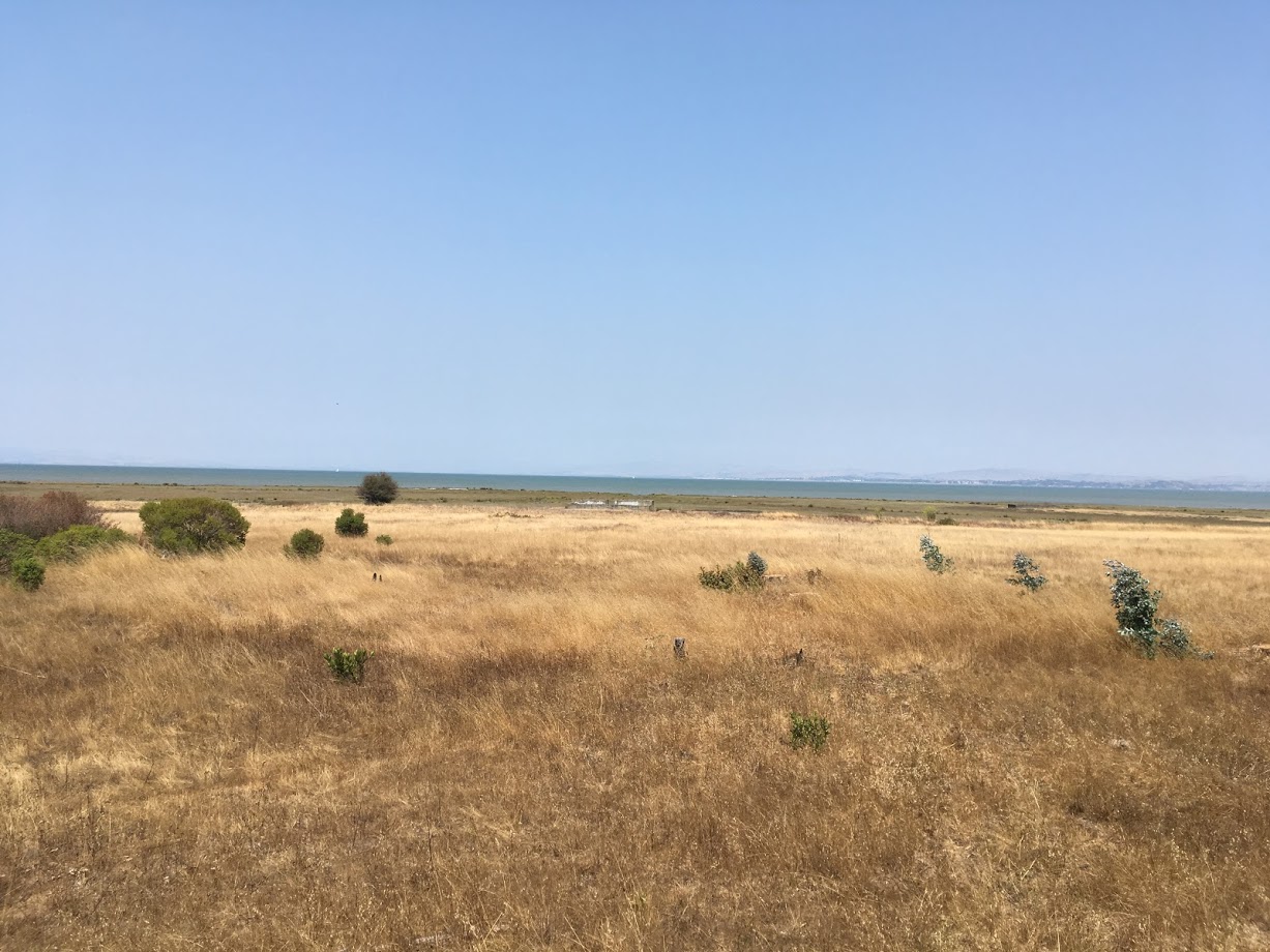 and a field...
|
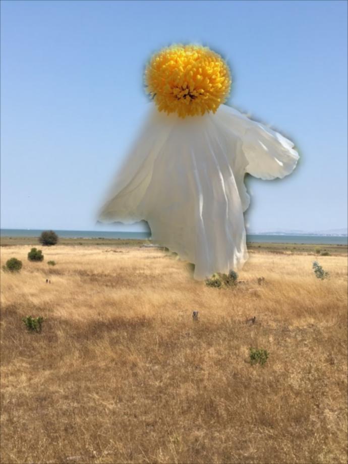 make an eggflower field!
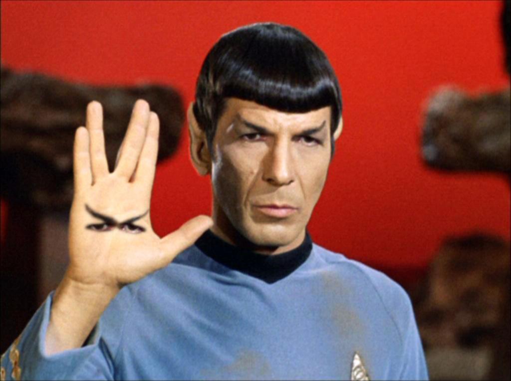
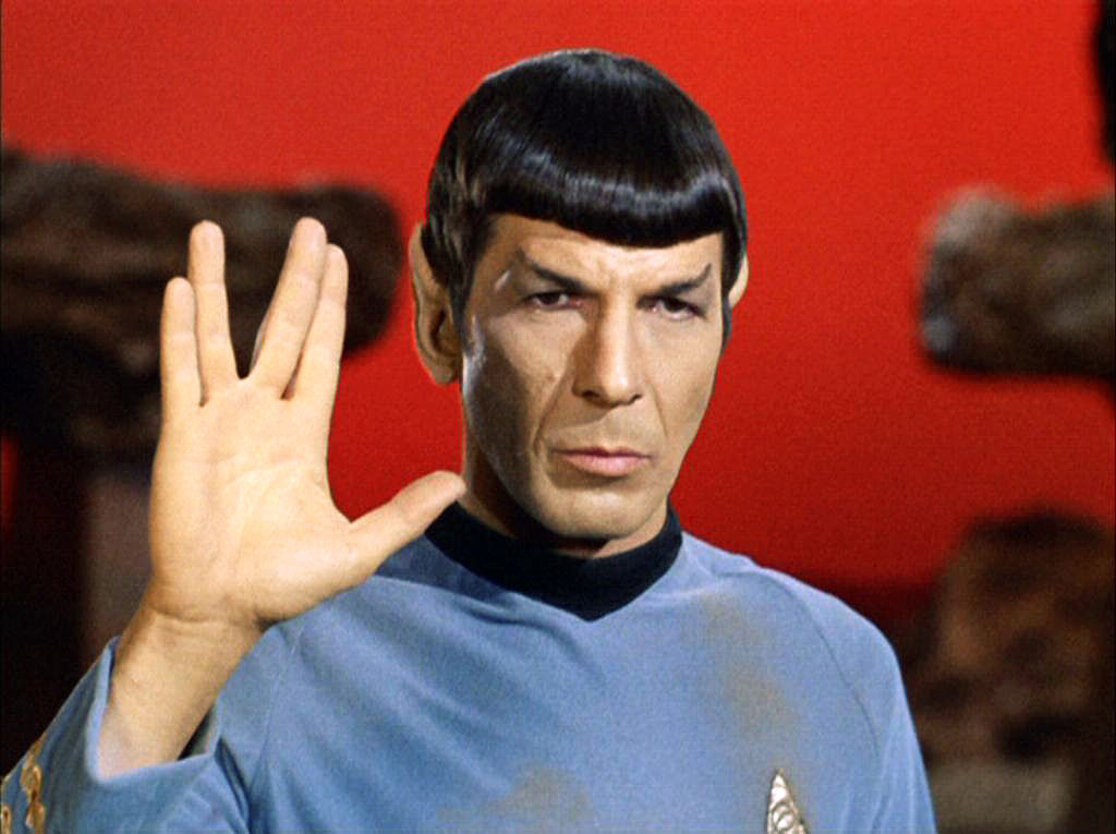 I found this on google images under commercial and other licenses so I don't think CBS/Viacom will come after me?
|
|
The only bells and whistles I could implement were producing the images in color. I started with using grayscale, then applied it to the rest of them.
I think the most interesting thing I learned in this project (and with this class in general) is the 'aha' moment when I learn or implement something similar to what I've used in
GNU GIMP or photoshop or something-- in this project, it was the case of Gaussian filters and edge blending (mainly with the multiresolution spline). I also think it's fascinating
how 'hidden' images can exist in the form of low frequency and high frequency components of an image, like with the Mona Lisa or the Salvador Dali painting.