The goal of this project is to show how image filters and frequencies can
create a lot of cool image results such as image blurring, sharpening, and
straightening. We will also see how these functions can be combined to
create hybrid and blended images.
Part 1: Fun With Filters
Image filters can be thought of as functions that take in image as an
input and return a new image as an output. One such filter is a Gaussian
filter which takes in an input image and returns a blurred version of it.
Some functions we will be applying to our images in this project are
gradients. Gradients tell us how much a part of an image in changing with
respect to a direction. This can be calculated by taking the partial
derivative of the image with respect to
x (the horizontal direction) or y (the vertical
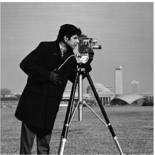
direction). Let us apply this to an image shown below:
Cameraman
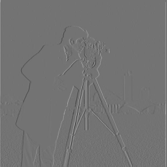
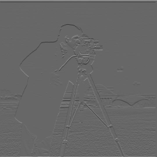
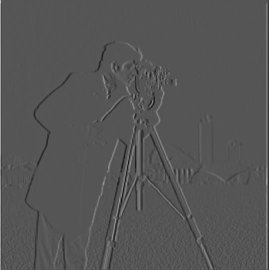
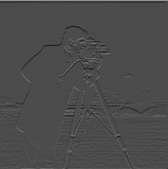
We can take the partial derivative in x and y of the
image by convolving it with finite difference operators
D_x = [1, -1] and D_y = [1, -1]^T respectively. The
results are shown below:
X Gradient
Y Gradient
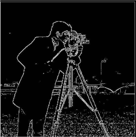
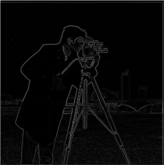
We can combine these gradients to get the gradient magnitude of the image,
which we will use to find the edges of the image. To compute the gradient
magnitude, we simply square the result of our x gradient and
y gradient, add them together, and take the square root of the
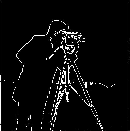
sum (magnitude = sqrt((dx^2) + (dy^2))). After taking the
gradient magnitude, I binarized it by making all pixel values that were
greater than a threshold of 0.12 one, and zero otherwise. This allows us
to see the edges of the image more clearly while suppressing the noise.
The gradient magnitude of the image is shown on the left and the edge
image is shown on the right.
Gradient Magnitude
Binarized Gradient Magnitude
Part 1.2: Derivative of Gaussian (DoG) Filter
Notice that despite binarizing our gradient magnitude image, a lot of high
frequency noise is still present in our edge image. This issue can be
solved by running our image through a low-pass filter, which keeps the low
frequencies of the image and attenuates the high frequencies (this also
blurs the image). We can do this by convolving our image with a Gaussian
filter and repeating the same process that was performed earlier. In my
implementation, I used a 3 x 3 Gaussian filter with
σ = 1.
X Gradient
Y Gradient
Gradient Magnitude
Binarized Gradient Magnitude
We can see that the biggest difference between the above edge image and
our previous edge image is the high frequency noise from the grass and
background were attenuated with the Gaussian filter. The edges of the man
and the camera have become more defined.
Instead of convolving our image twice, we can make calculations more
efficient by combining our finite difference operators with our Gaussian
filter and get away with convolving our image only once. This is possible
due to the associative property of convolutions. As expected, this gives
us the same results as earlier. The combined filters and edge image are
shown below:
X Gaussian Gradient
Y Gaussian Gradient
Binarized Gradient Magnitude
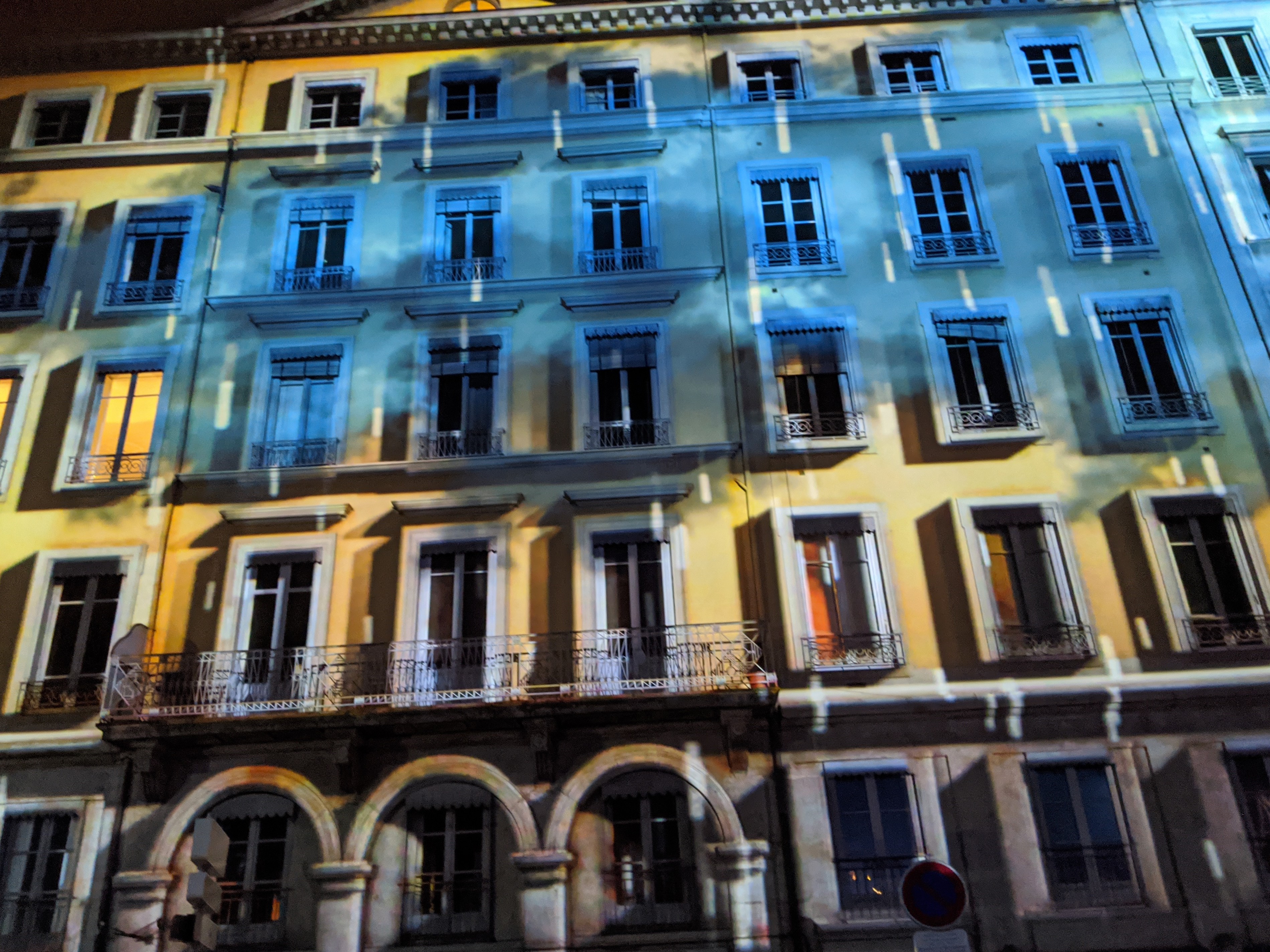
Part 1.3: Image Straightening
Sometimes when we take pictures, the pictures don't come out straight.
Manually rotating the image to get the right position is too much work.
Thankfully, we can use our knowledge of gradients to automate the image
straightening process! In my implementation, I rotated an input image by
various angles in a predefined range and chose the rotation that had the
most number of horizontal and vertical lines. To account for sizing
differences when rotating, I did not resize the image after rotation and
cropped the center of the image to perform my calculations on. I counted
the number of horizontal and vertical lines by computing the gradient
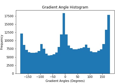
angle of each pixel in the image with the formula:
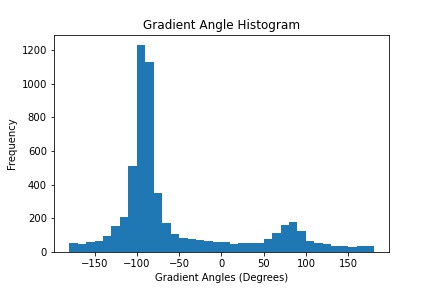
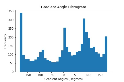
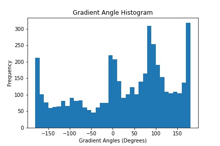
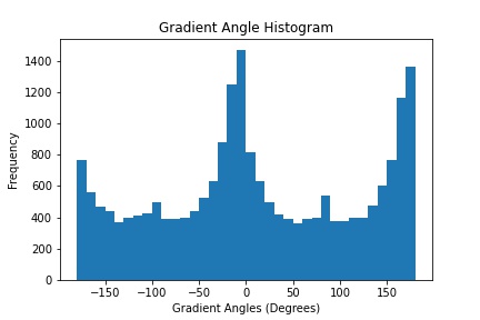
θ = atan2(dy, dx) * 180 / π. The results of my implementation
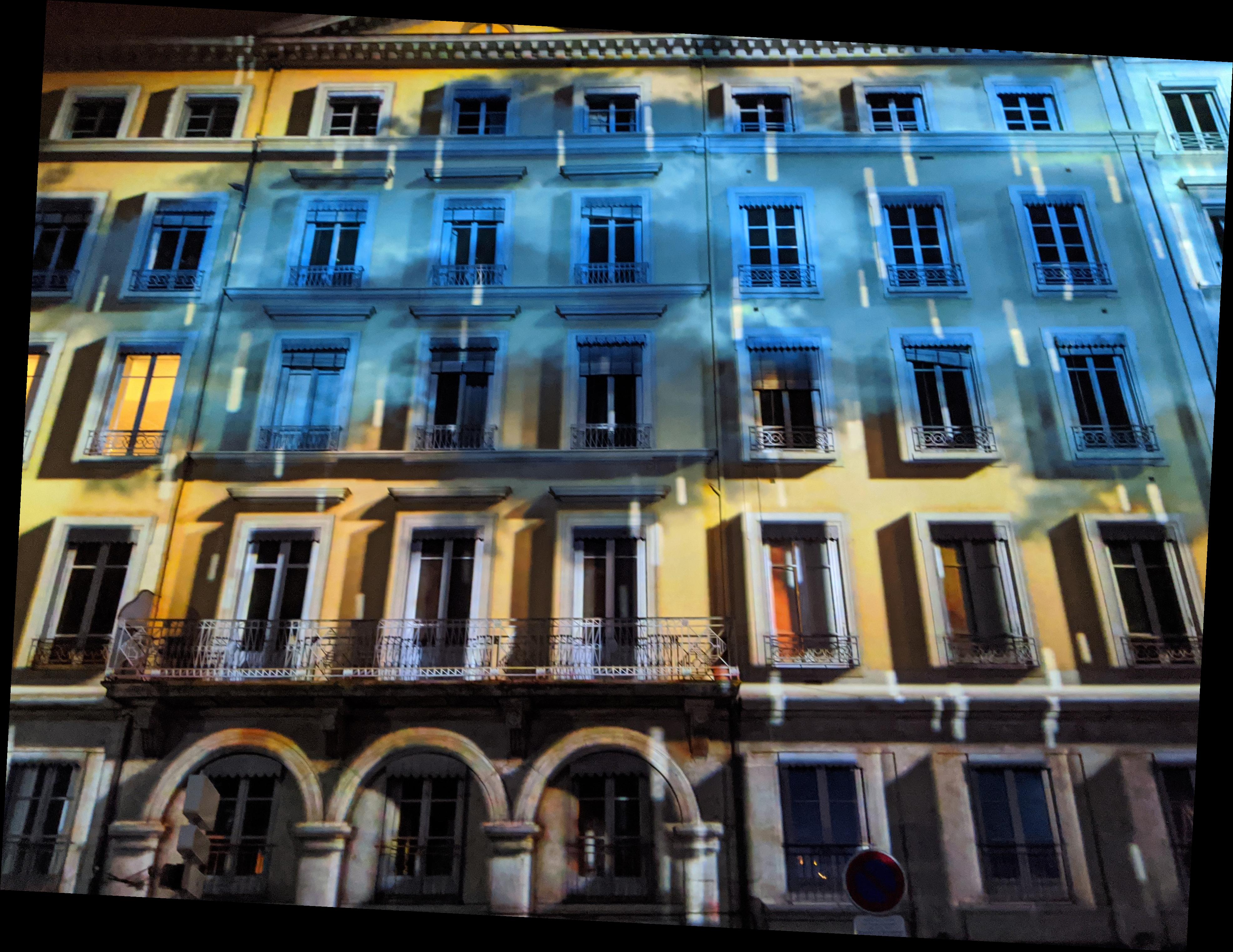
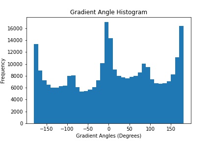
on several images are shown below. For each image, the histogram next to
it depicts the number of gradient angles the cropped image contains before
and after straightening.
Before Straightening - Facade
After Straightening (Rotated -3°)
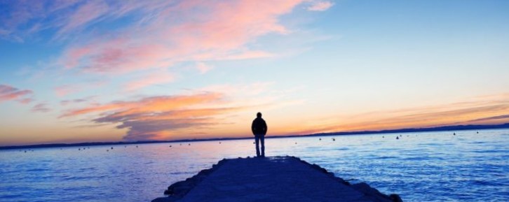
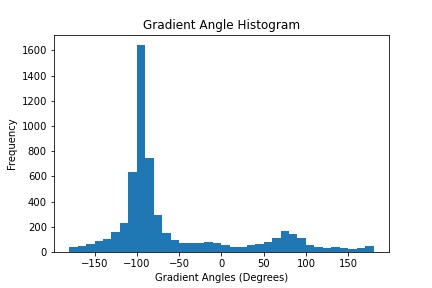
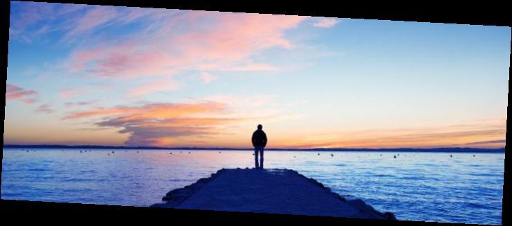
Before Straightening - Horizon
After Straightening (Rotated -2°)
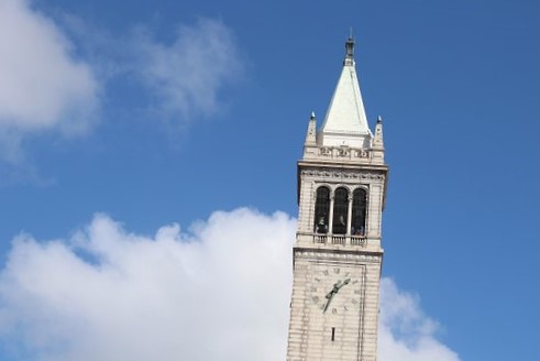
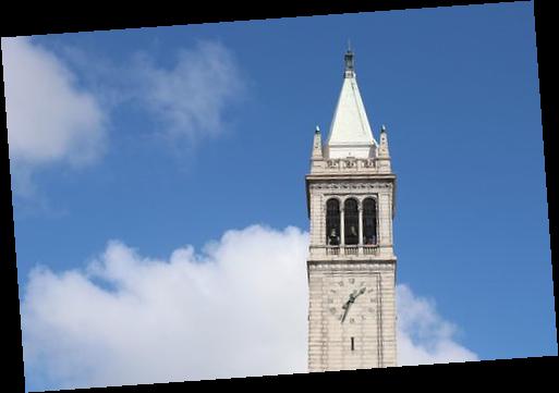
Before Straightening - Campanile
After Straightening (Rotated -4°)
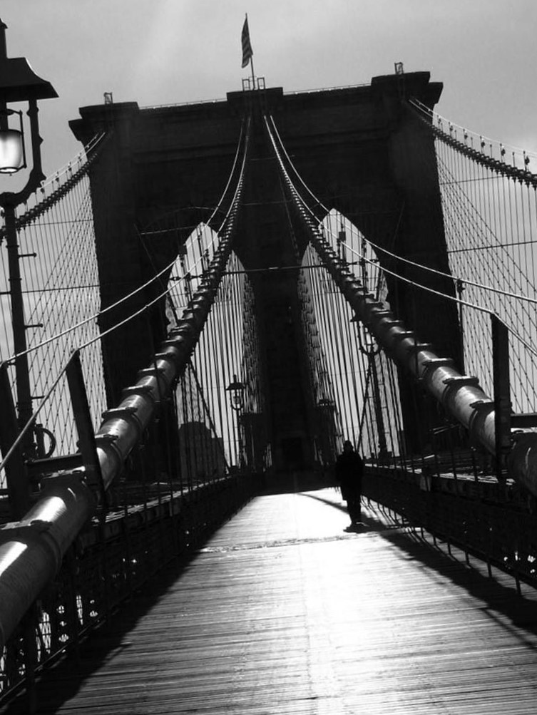
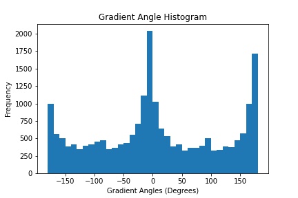
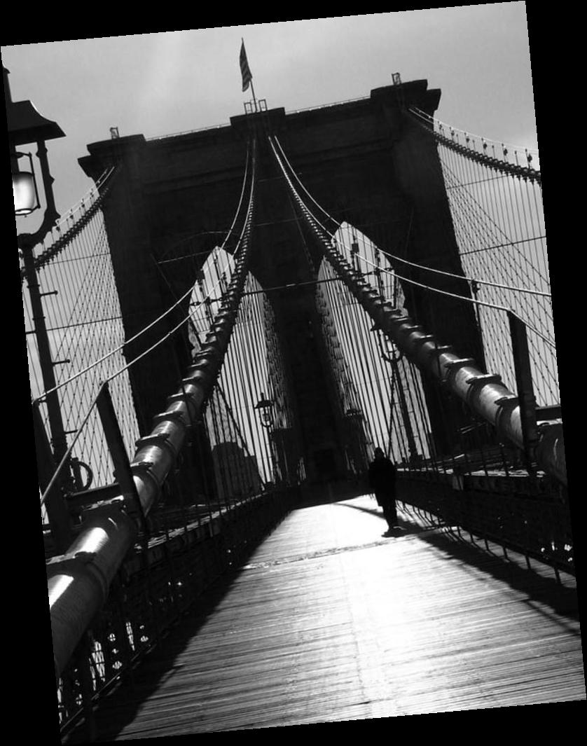
Before Straightening - Brooklyn Bridge
After Straightening (Rotated 5°)
As you can see, my implementation failed on the last image above. This is
due to many of the edges of the Brooklyn Bridge image being
non-perpendicular such as the wires connecting the bridge. By trying to
straighten the image, my program instead attempted to minimize the number
of non-perpendicular edges which results in the unstraightened image.
Part 2: Fun With Frequencies
In this part of the project, we will show how manipulating image
frequencies can sharpen images and create hybrid/blended images!
Recall earlier that we used a Gaussian filter to keep the low frequencies
of an image. To get the high frequencies of an image, we simply take our
filtered image and subtract it from our original image. The high
frequencies of an image tell us how "sharp" an image is. By scaling the
high frequencies of an image, we can automate sharpening our own images!
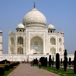
In my implementation, I first blurred an input image with a Gaussian
filter of size 5 x 5 and σ = 2 then subtracted it
from the original image to obtain the high frequency image. Next, I scaled
the high frequency image by some alpha value (α) and then added that
result back into our original image to obtain the sharpened image. This
process can be seen in the images below:
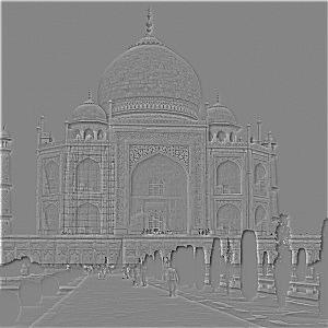
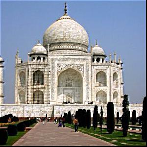
Original Image (Taj Mahal)
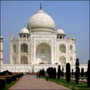
Blurred Image
High Frequency Image (Grayscale for visibility)
Sharpened Image
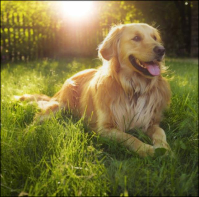
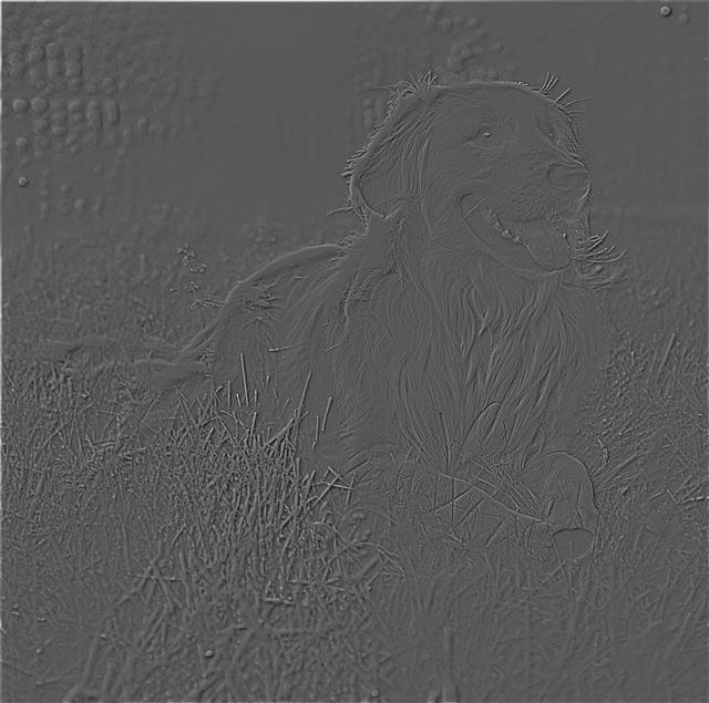
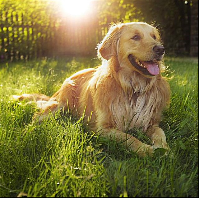
Original Image (Golden Retriever)
Blurred Image
High Frequency Image (Grayscale for visibility)
Sharpened Image
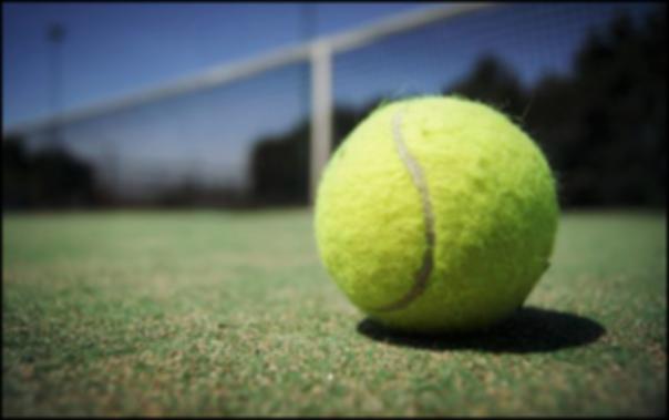
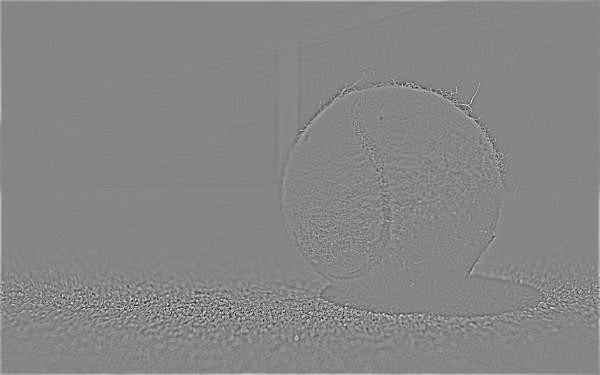
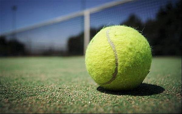
Original Image (Tennis Ball)
Blurred Image
High Frequency Image (Grayscale for visibility)
Sharpened Image
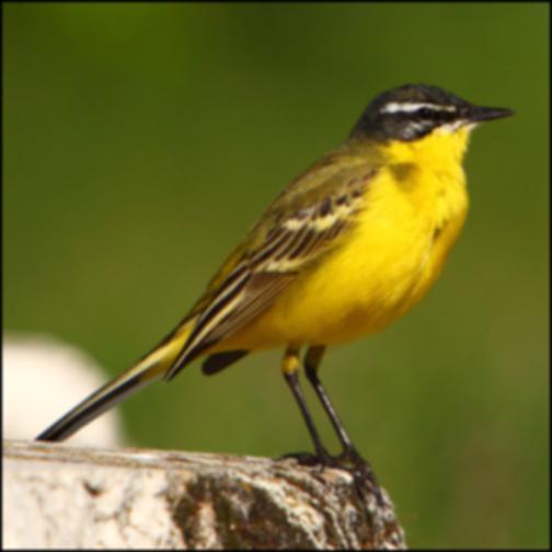
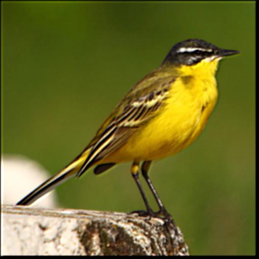
Let's see what happens when we take an already sharp image, blur it, then
sharpen it again. The result is shown below:
Original Sharp Image (Bird)
Blurred Image
Sharpened Image
As you can see, the final sharpened image is not the same as the original
sharp image. This is because when blurring the input image with the
Gaussian filter, we lost some of the high frequency components that were
contained in the original image. Although we increased the intensity of
the remaining high frequency components in our output, we still lose some
high frequency information which is why the output image is not the same
as the input image.
Similar to our gradient magnitude image, we can make our calculations more
efficient by utilizing convolution properties. Currently, our sharpening
calculations can be modeled by the following formula:
image + α(image - image ∗ filter). This formula can be
rewritten as
(1 + α) * image - α * image ∗ filter = image ∗ ((1 + α) * e - α *
filter), where e is the unit impulse.
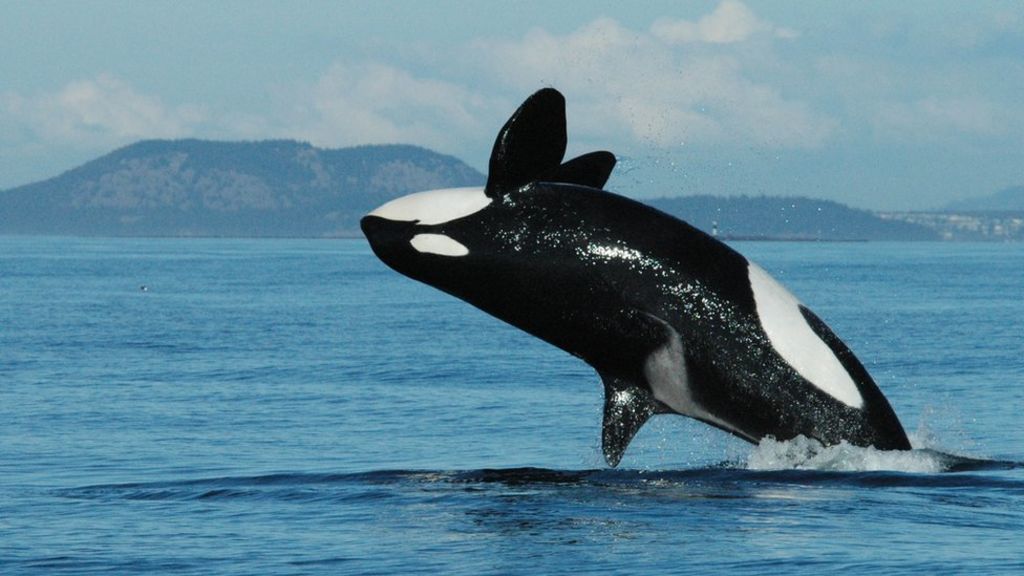
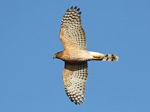
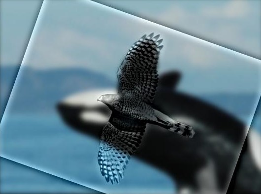
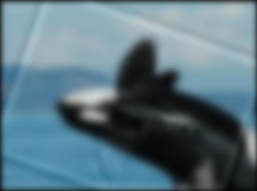
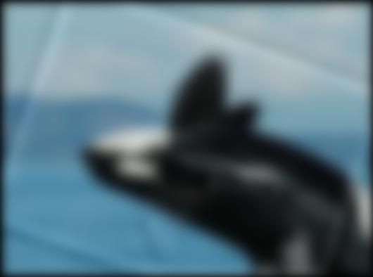
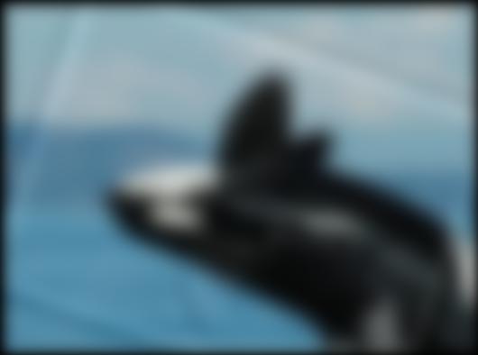
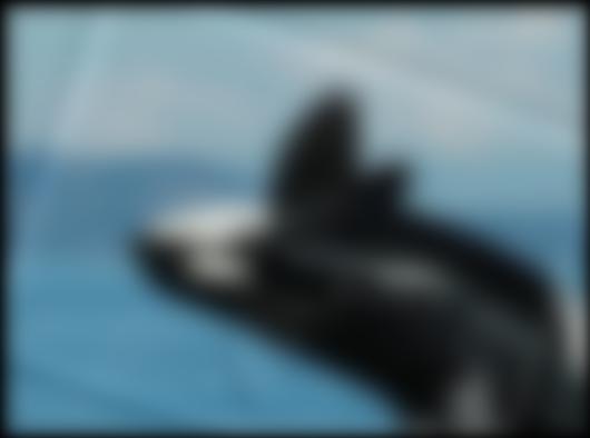
Part 2.2: Hybrid Images (Bells & Whistles)
In addition to using frequencies to sharpen images, we can also use them
to create hybrid images. In a hybrid image, a user sees a high frequency
image at close viewing angles but sees a different low frequency image at
farther viewing angles. Essentially, this allows two images to be
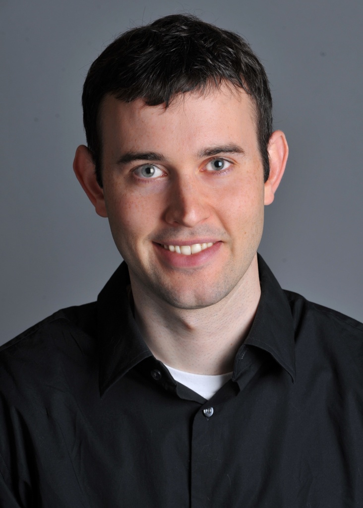
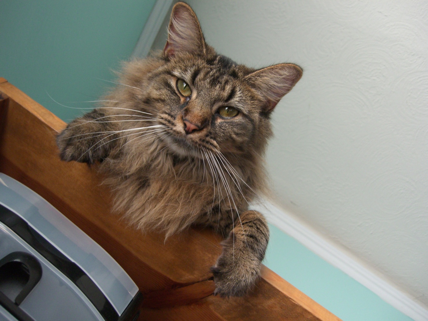
encompassed into one. To create a hybrid image, I first aligned two input
images at some chosen reference point. Next, I separated the color
channels of each image and separated the low frequency image from the
first image and the high frequency image from the second image. Finally, I
combined the two frequencies together and stacked the color channels at
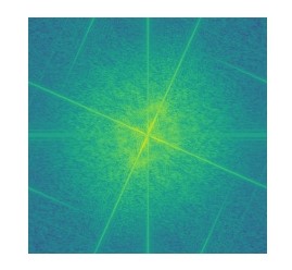
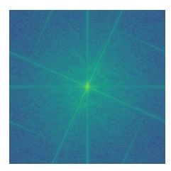
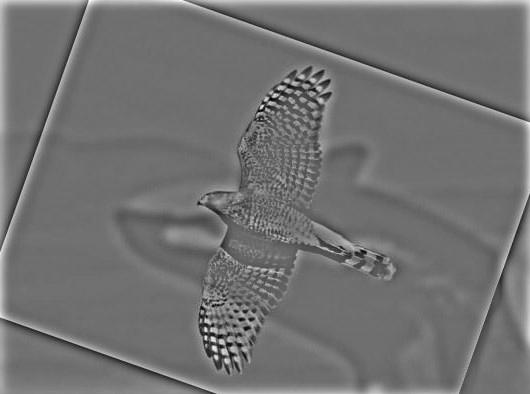
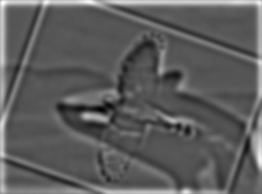
the end to create a colored hybrid image. The first set of images
displayed below has a frequency analysis of the process which shows the
Fourier transform of the input images, the filtered images, and the resulting
hybrid image. (For bells & whistles, I used color to enhance the effect of
the hybrid images. Through experimentation, I found that only adding color
to the low frequency image makes for an interesting result. Adding color
to the high frequency image makes little difference because the human eye
cannot see high frequency color well.)
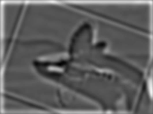
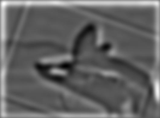
Whale
Hawk
Hybrid
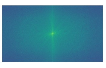
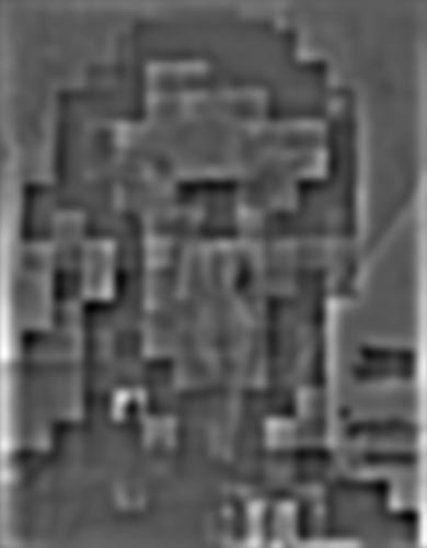
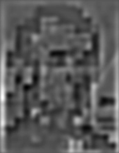
Fourier Transform Whale
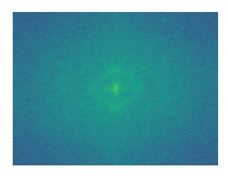
Fourier Transform Hawk
Low Frequency Whale Fourier Transform
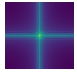
High Frequency Hawk Fourier Transform
Hybrid Fourier Transform
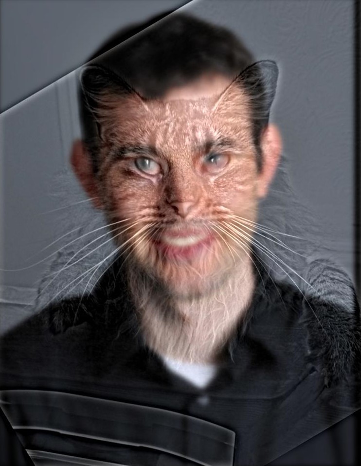
Derek
Nutmeg
Hybrid
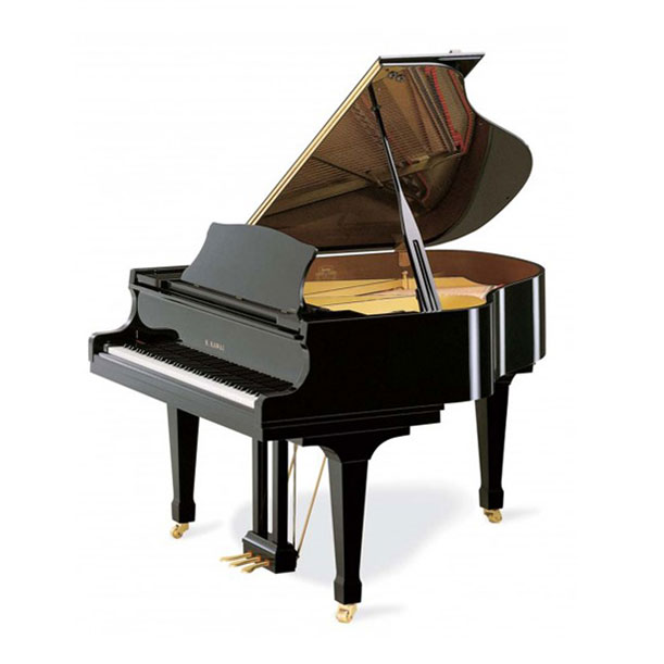
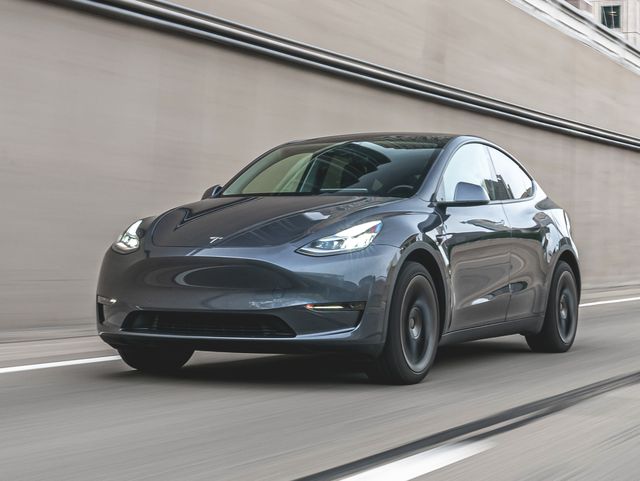
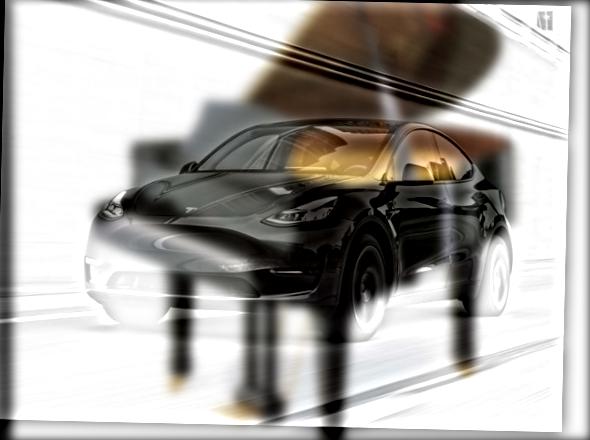
Piano
Tesla
Hybrid
The above hybrid is an example of a failure case. The piano and Tesla did
not align particularly well, resulting in the Tesla image being hard to
see at all viewing angles.
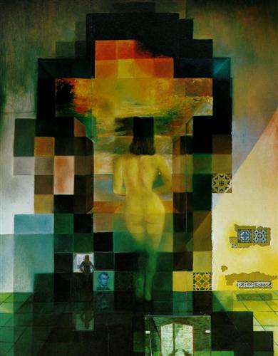
Part 2.3: Gaussian and Laplacian Stacks
Another function we can do with image frequencies is discovering the
structure of images at different resolutions. Recall that when applying a
Gaussian filter to an image, it isolates the low frequencies of that
image. Similarly, subtracting the low frequency image from the original
image gives us the high frequency image. In this section, we will be
implementing a Gaussian and Laplacian stack. In the Gaussian stack, my
implementation takes an input image and repeatedly filters it with a
Gaussian filter of size 30 x 30 with σ = 5 at 5
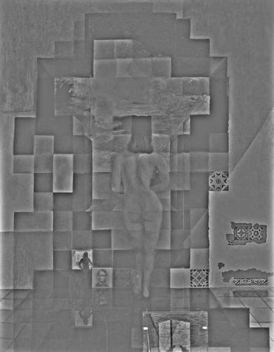
levels. For the Laplacian stack, I simply take a Gaussian filtered image
at a single level and subtract it from the Gaussian filtered image at the
previous level. This implies that we will need to calculate an extra
Gaussian filtered image to create 5 Laplacian filtered images. The result
of this process on several hybrid images is shown below. You will notice
that the stacks reveal different frequency structures at each level. The
Laplacian stack has been converted to grayscale for better visibility.
Original (Lincoln in Dalivision)
Level 1 (Gaussian)
Level 2
Level 3
Level 4
Level 5
Level 1 (Laplacian)
Level 2
Level 3
Level 4
Level 5
Original (Hybrid)
Level 1 (Gaussian)
Level 2
Level 3
Level 4
Level 5
Level 1 (Laplacian)
Level 2
Level 3
Level 4
Level 5
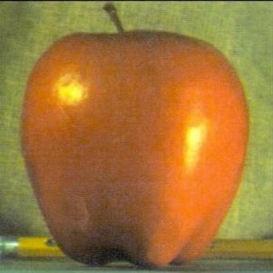
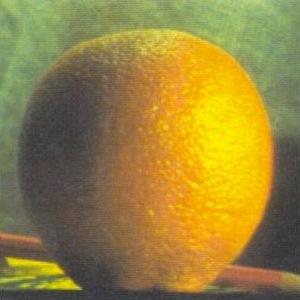
Part 2.4: Multiresolution Blending (Bells & Whistles)
The coolest part of image frequencies is image blending. This part of the
project blends two images such that there is a smooth joining between
them. To generate this blend, my implementation first separates the color
channels of my input images and takes the Laplacian stacks of the parts of
the two images to be blended together. Next, I create a mask of the image
and apply the Gaussian stack to it with a Gaussian filter of size
30 x 30 and σ = 5. This mask is a crucial part of
the implementation that creates a seamless join between the two images.
After creating the stacks, each level of all three stacks are combined
with the following formula:
blended level = Laplacian level of image 1 * Gaussian level of mask +
(1 - Gaussian level of mask) * Laplacian level of image 2
Once we have created our blended levels, we will combine all blended
levels to form the final blended image and stack the color channels to
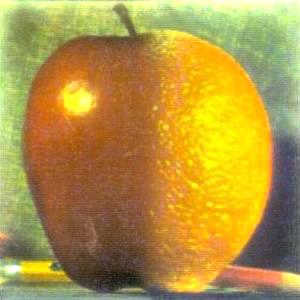
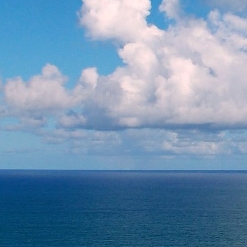
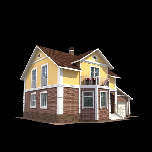
produce the colored image. See below for some cool blended images!
Apple
Orange
Mask
Blended Image
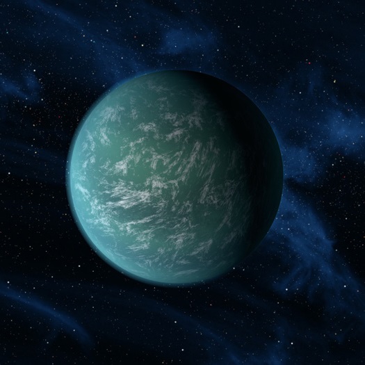
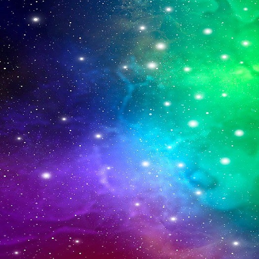
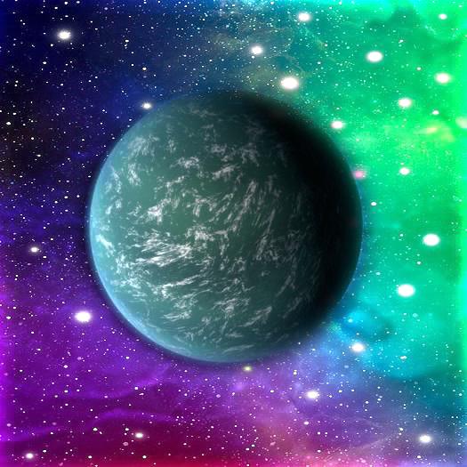
Kepler-22b
Space Background
Mask
Blended Image
Ocean
House
Mask
Blended Image
Final Thoughts
This project was very exciting to work on and allowed me to learn a lot
about how we can manipulate images using only filters and image
frequencies. My favorite thing that I learned was how simple yet
extraordinary Gaussian filters are when you apply them to images. In every
part of this project, we have used Gaussian filters in some way to create
the final image that we wanted. By far, the coolest thing that I learned
is how to blend images to create interesting and crazy effects. This has
made me realize that the field of computer vision is vast and there is
always something to learn!