CS 194-26 Fall 2020
Project 2: Fun with Filters and Frequencies!
Brian Wu
Part 1: Fun with Filters
Part 1.1: Finite Difference Operator
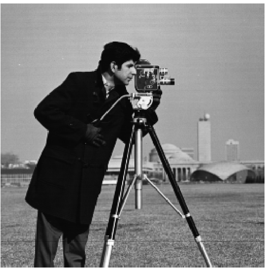
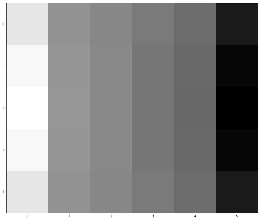
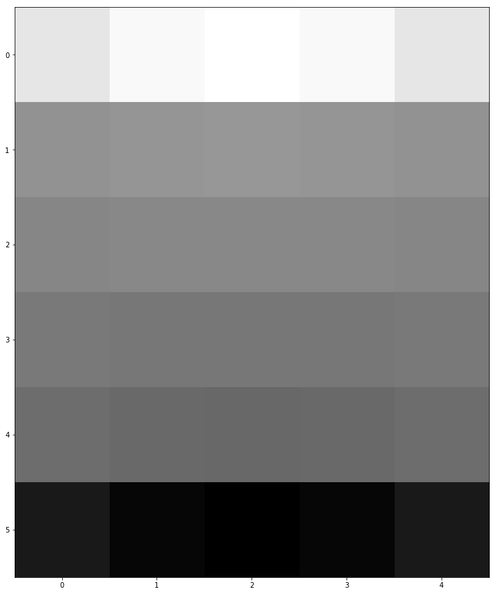
The general idea for computing the gradient magnitude was as follows: in order to find the magnitude of the gradient at a particular point, we first need the value of the partial derivatives in the X and Y directions at that point. The approximation of the partial derivative in the X direction for our discrete images is simply the difference between current pixel and next pixel, since df(x,y)/dx is approximated by [f(x + 1, y) - f(x, y)]/1.
To concisely represent this operation, we use convolutions. In our case, for the X direction, if we want this difference we can convolve 2D array [[1, -1]] with the image (using same mode to preserve size), where the former acts as a filter. This is like cross-correlation except we flip our filter in X and Y direction before multiplying. We do similar actions for the Y direction, and we get two 2D arrays, each the same length and width as original image. To get the final result, we just compute the elementwise square root of sum of squares of X and Y partial derivatives. To represent this image in binary we set a threshhold on these values.
One final caveat is that our original image contains multiple channels for all the colors. To reduce this to a 2D representation we simply convert it to grayscale.
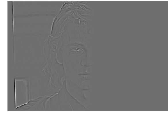
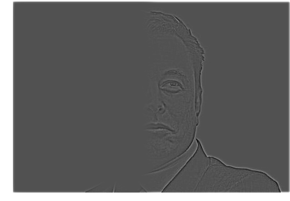
Part 1.2: Derivative of Gaussian (DoG) Filter
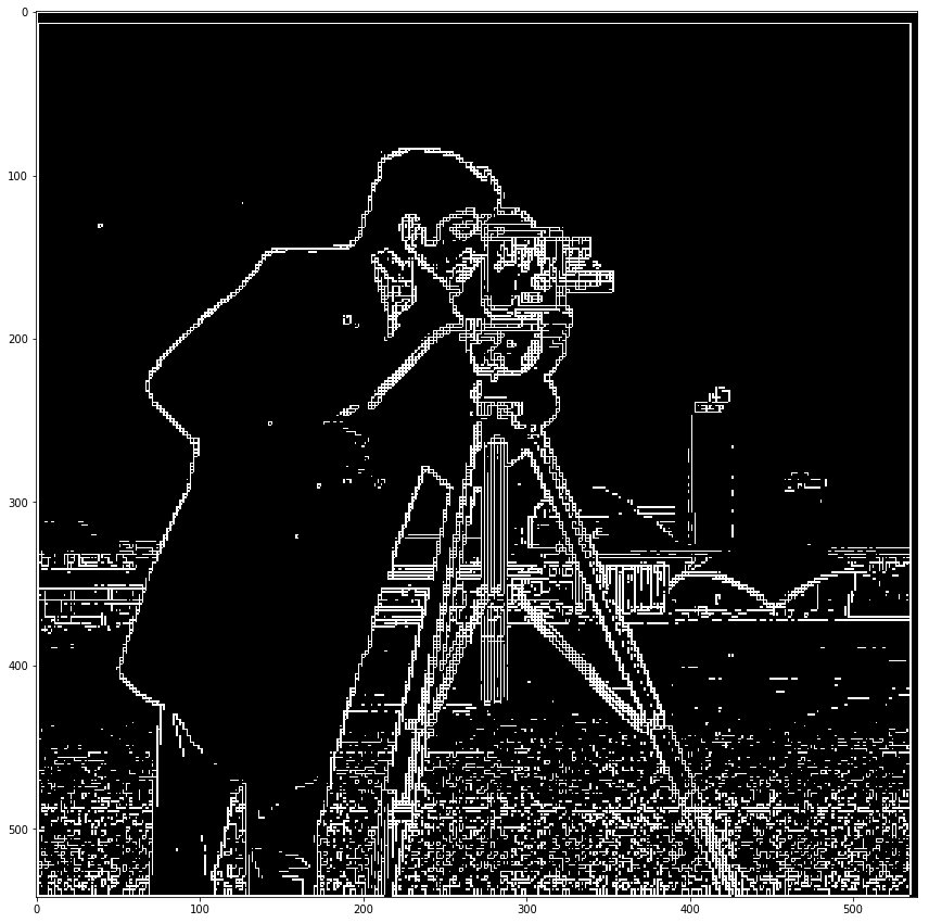
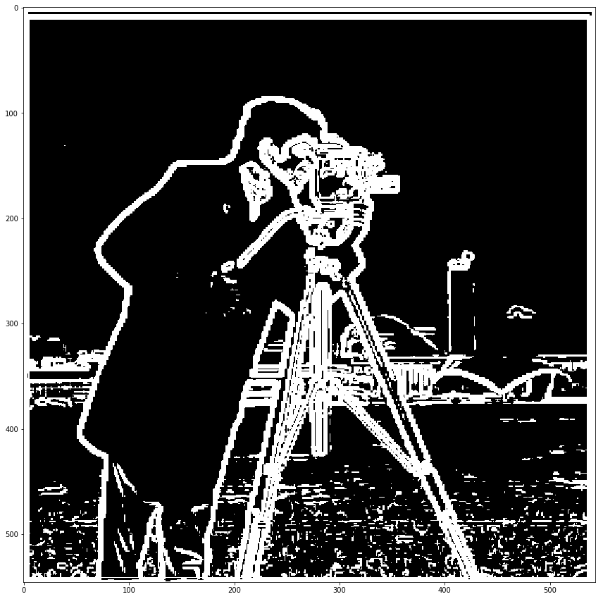
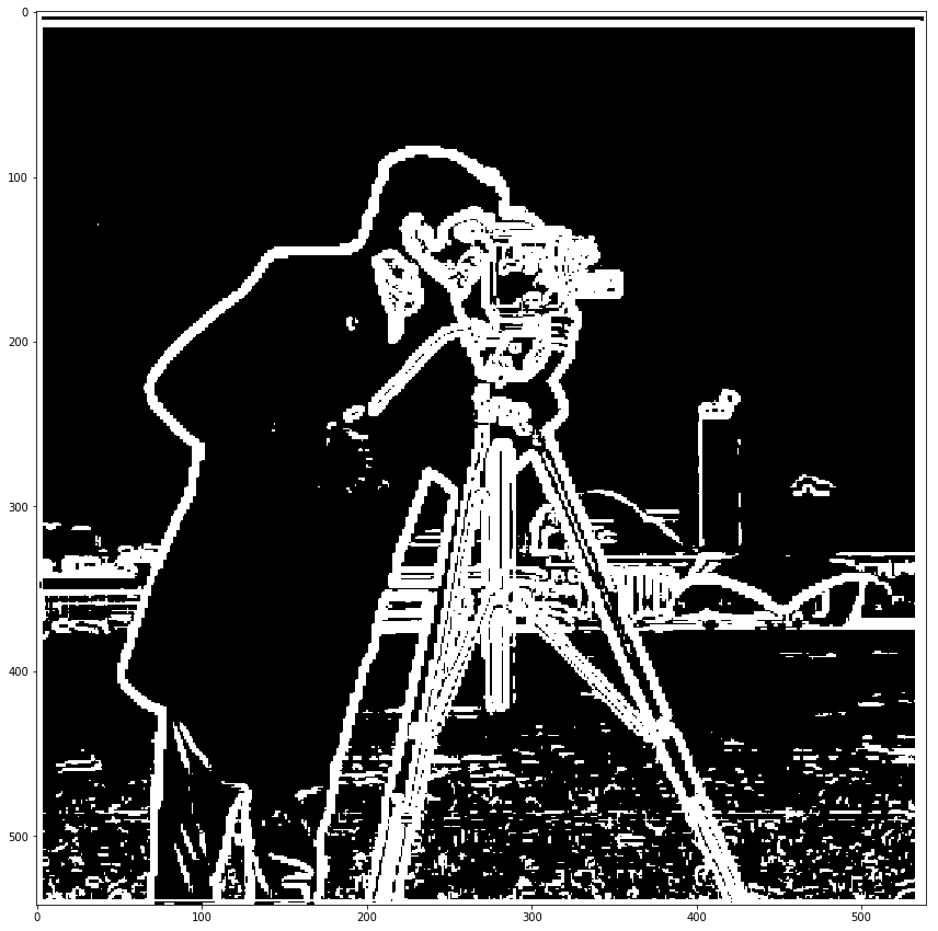
The differences between blurring the original image by convolving with a Gaussian filter before convolving with the difference operators are that the pre-blurred version give better edges, since the blurring results in significantly less noise by removing the sharpness of the non-edge noise, especially at the bottom of the image.
We also note that the result of convolving the Gaussian with the difference operators first, and using this DoG filter on the original image, results in the exact same output.

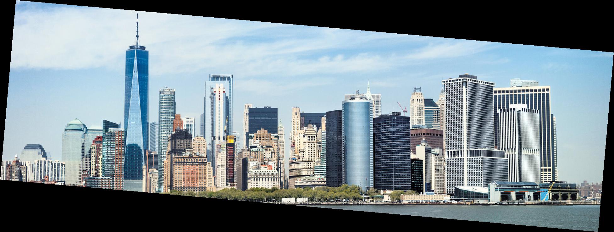
Part 1.3: Image Straightening
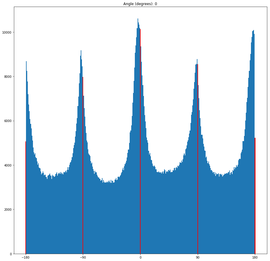
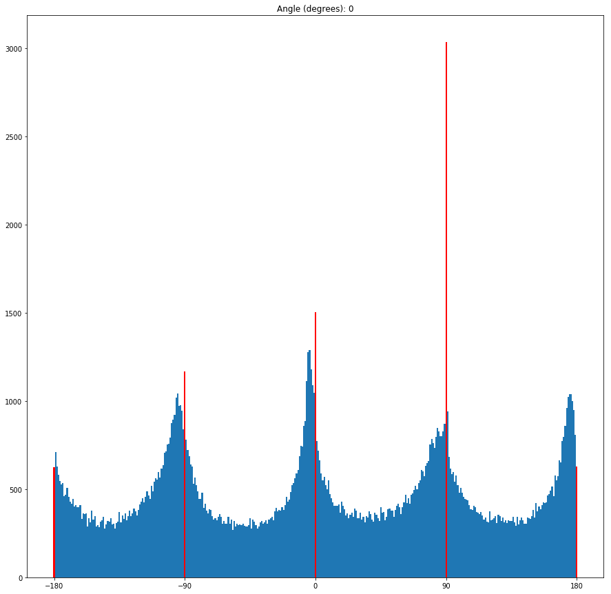
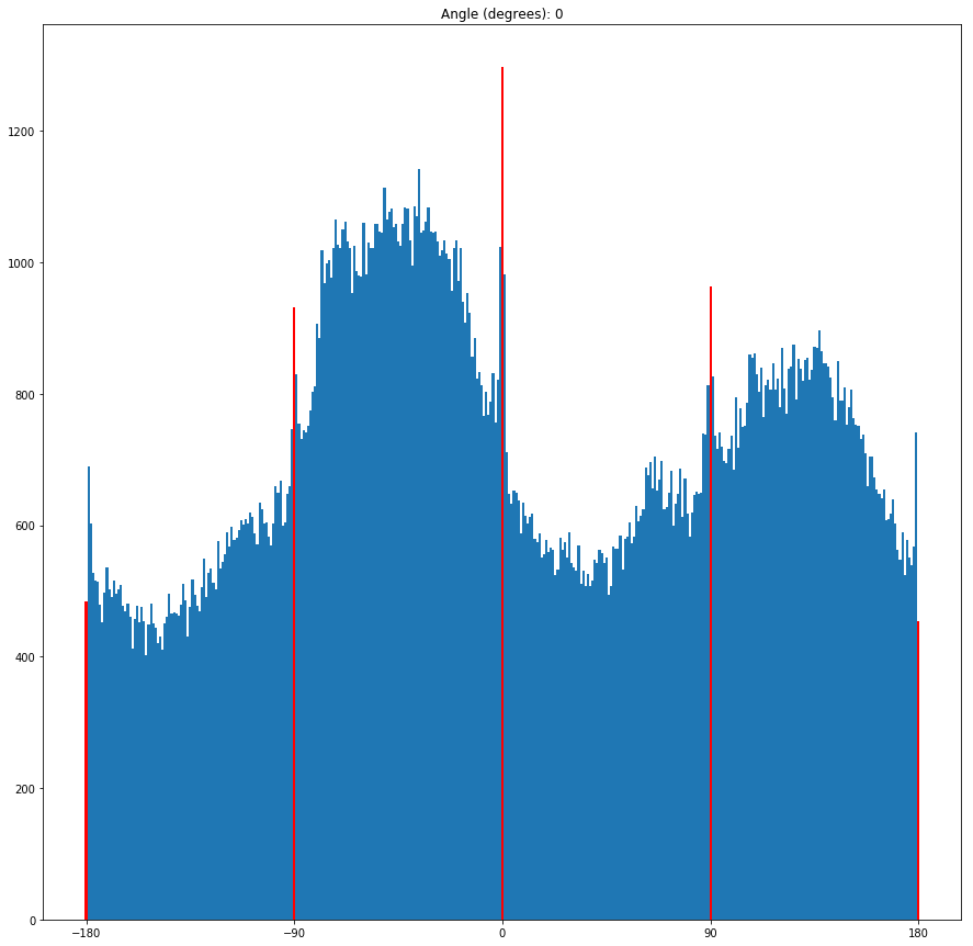
For this part, I attempt to straighten images by rotating them across some range, then computing a histogram of the orientation of all the edges. I then choose the rotation that gives the best percentage of horizontal and vertical edges, since we hope that a straightened image would have many horizontal and vertical edges.
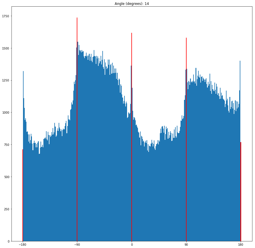
For visualization purposes, the histogram values for -180, -90, 0, 90, and 180 degrees have been highlighted in red. These values determined the amount of horizontal and vertical edges in my images.
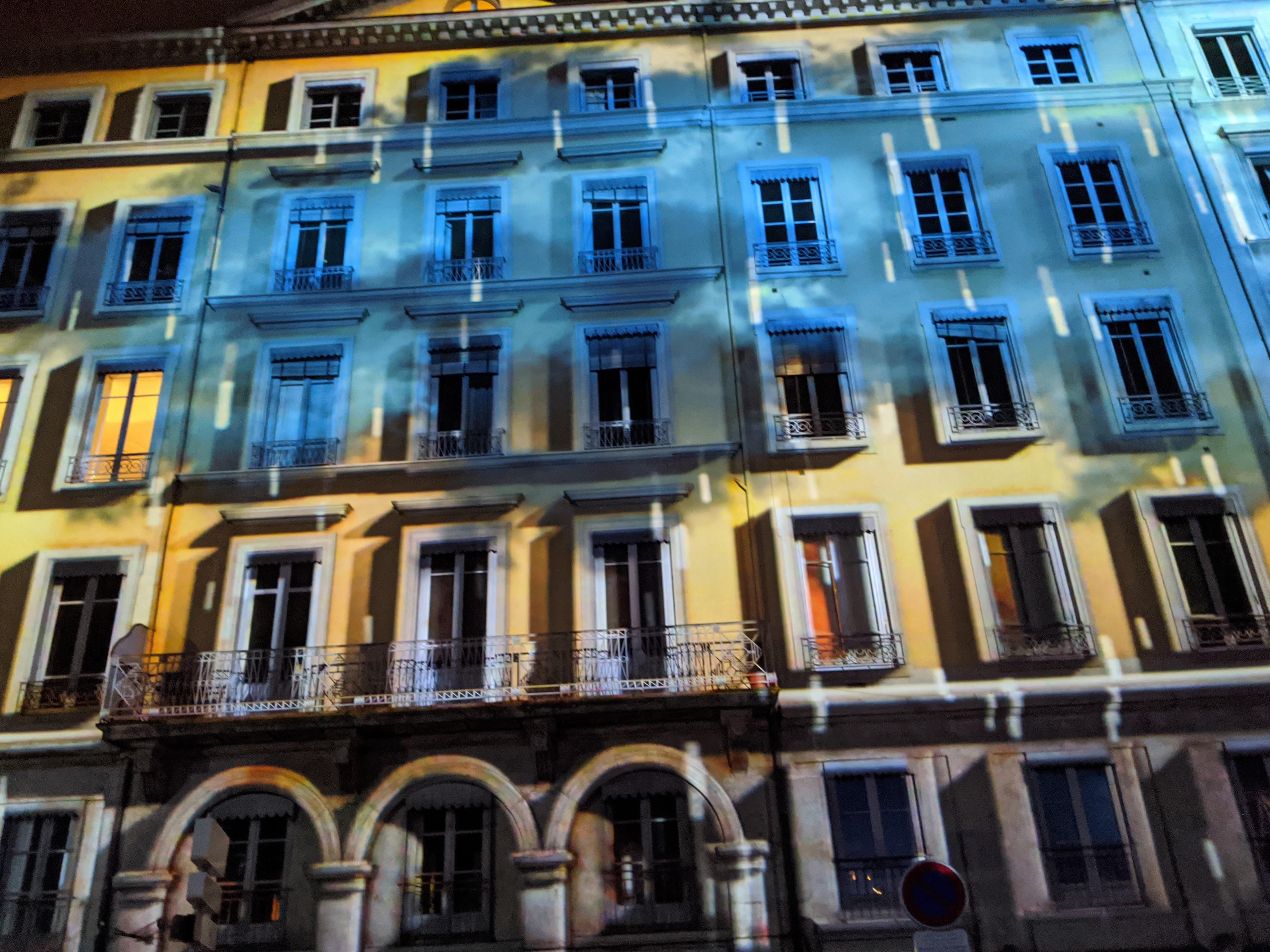
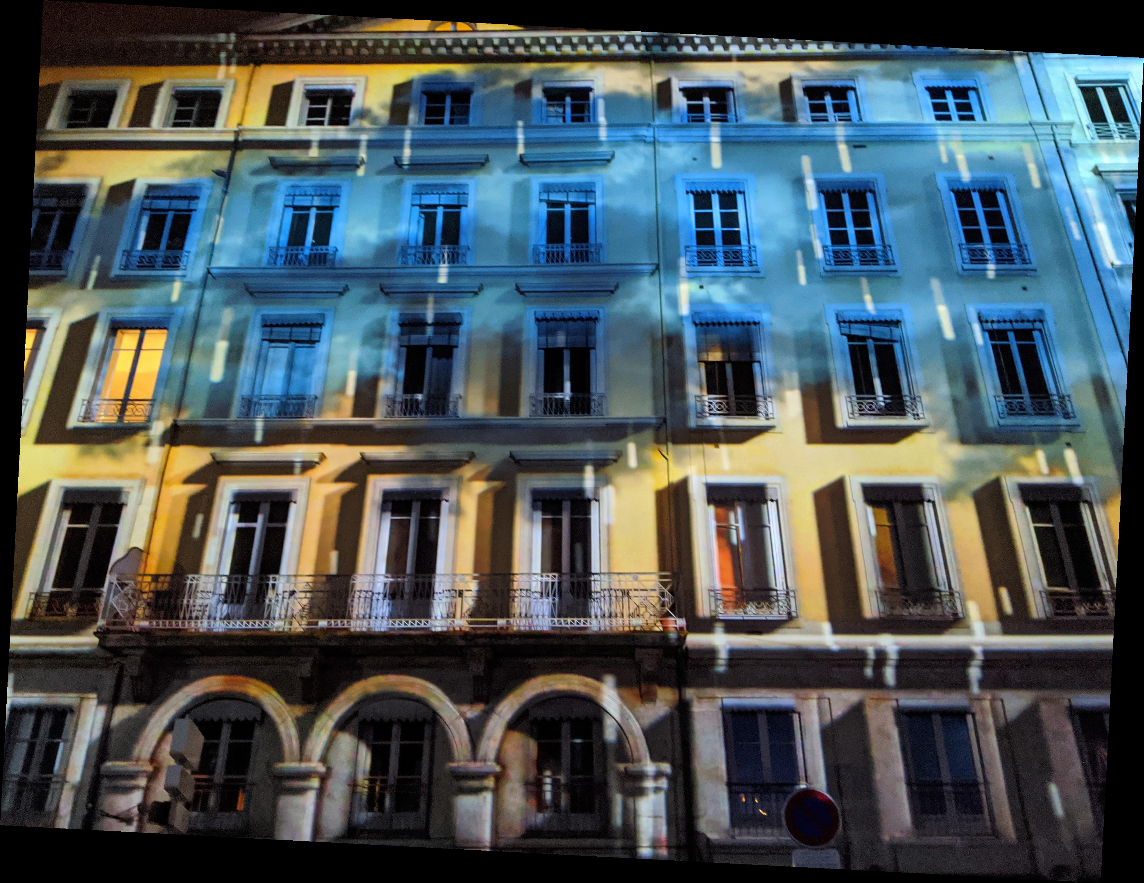
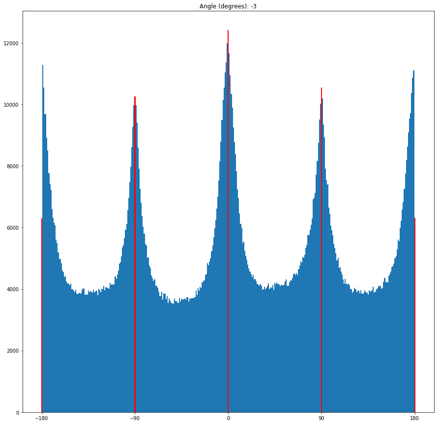
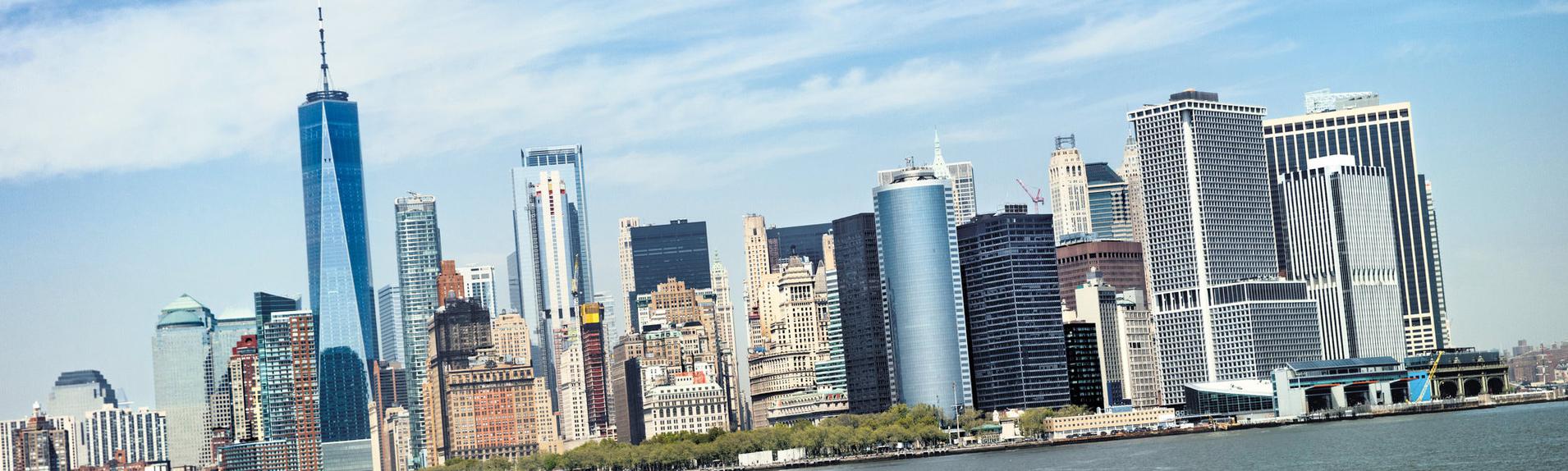
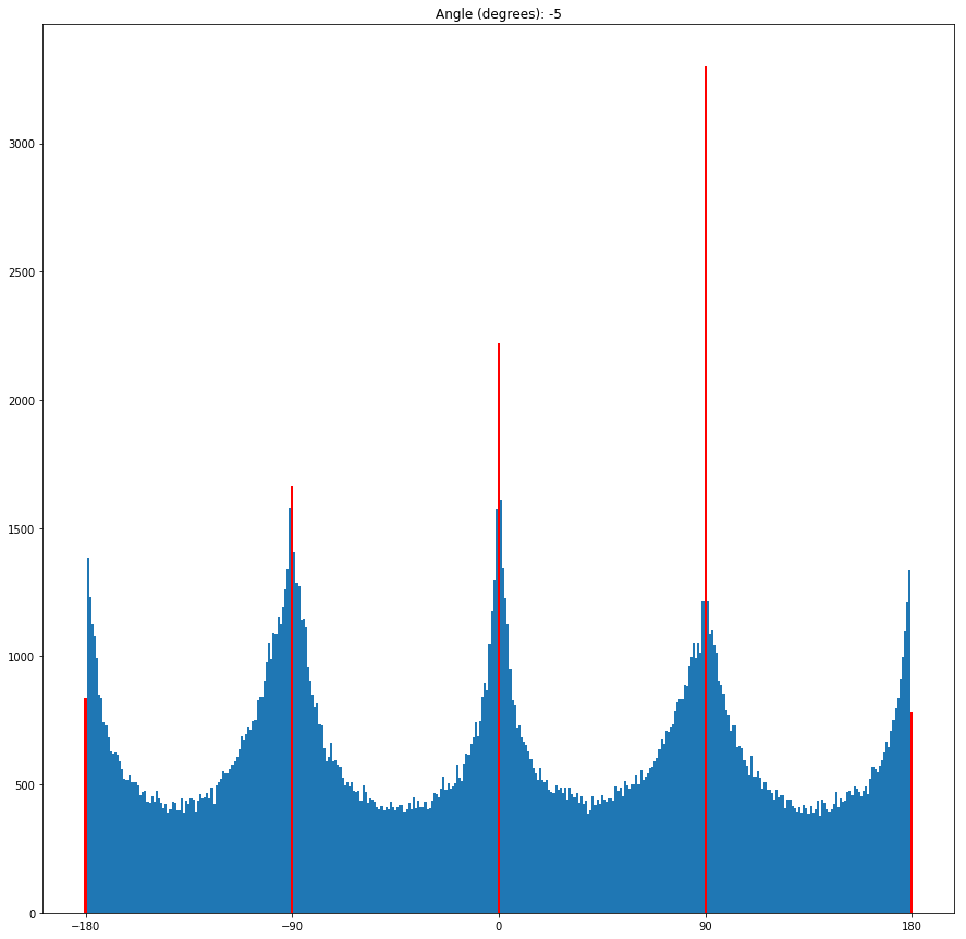
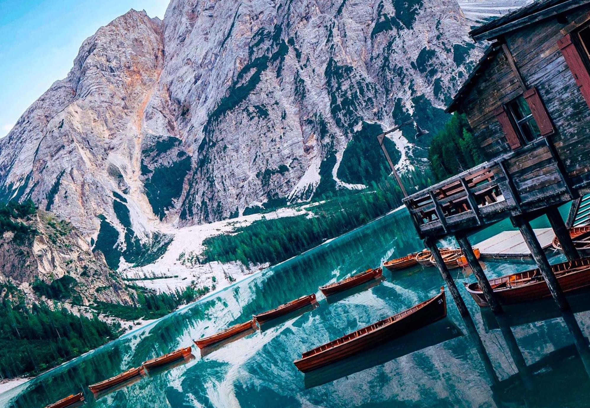
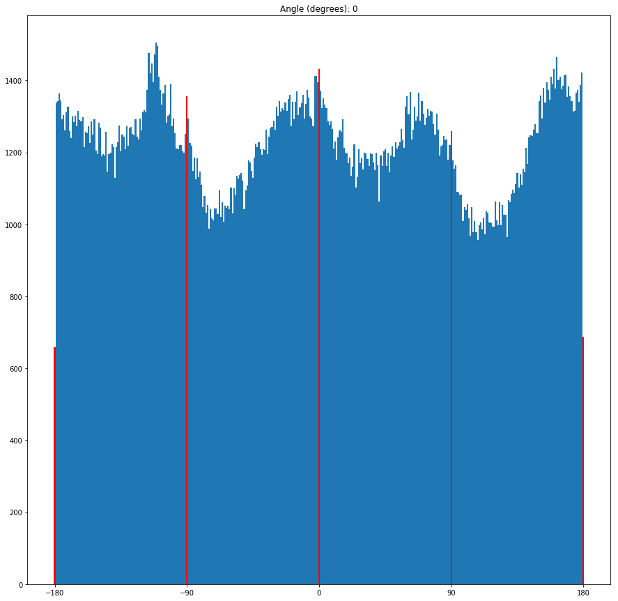
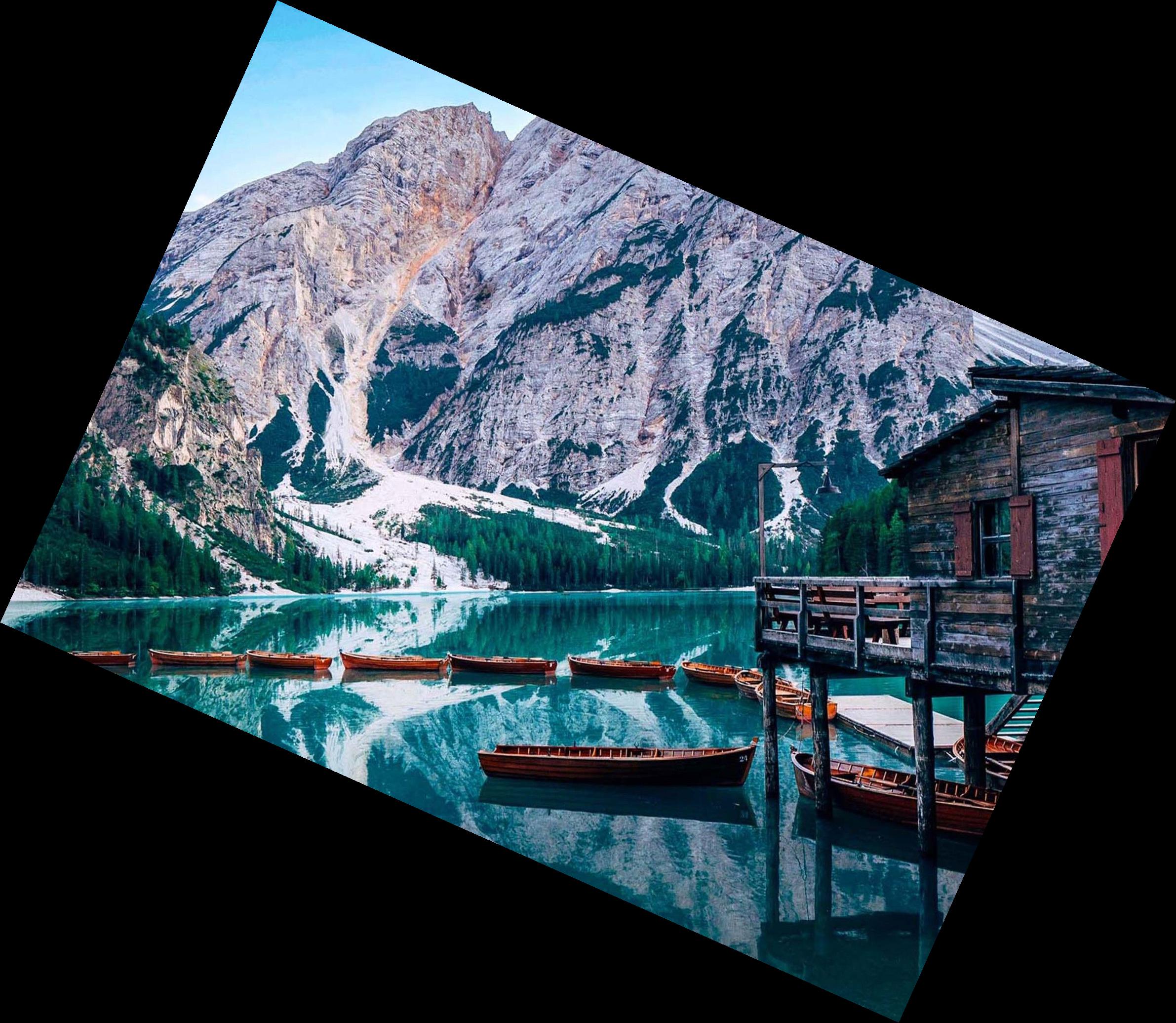
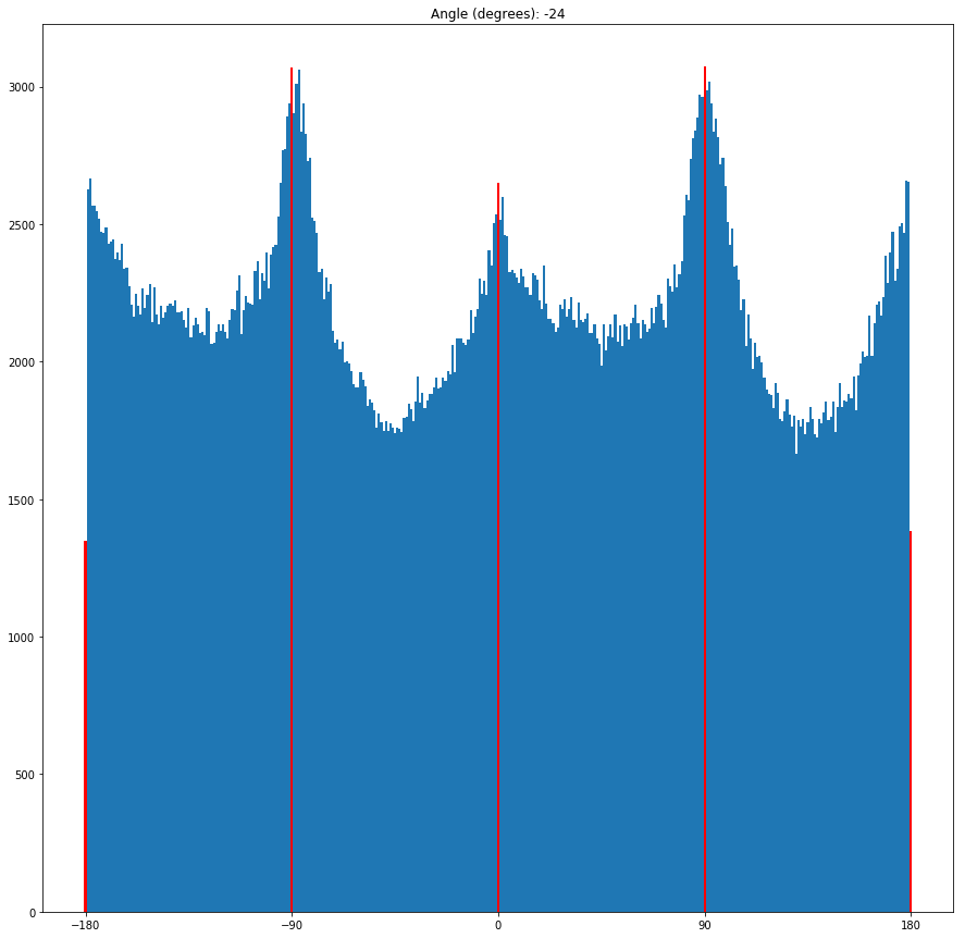
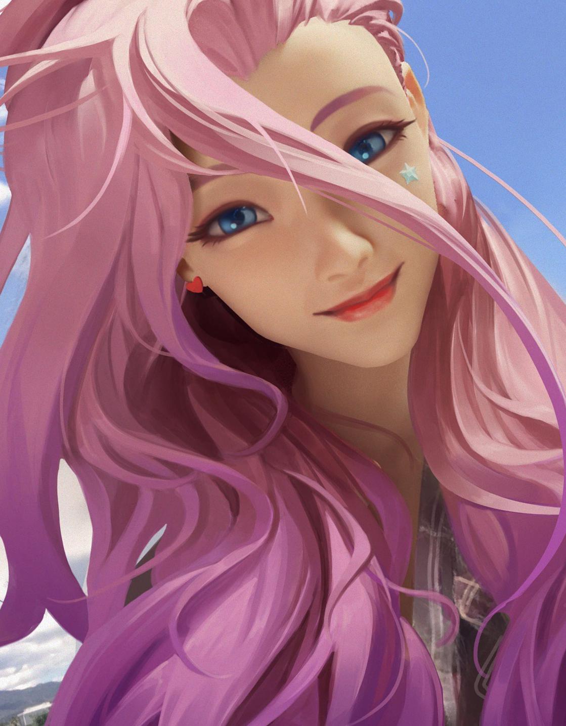
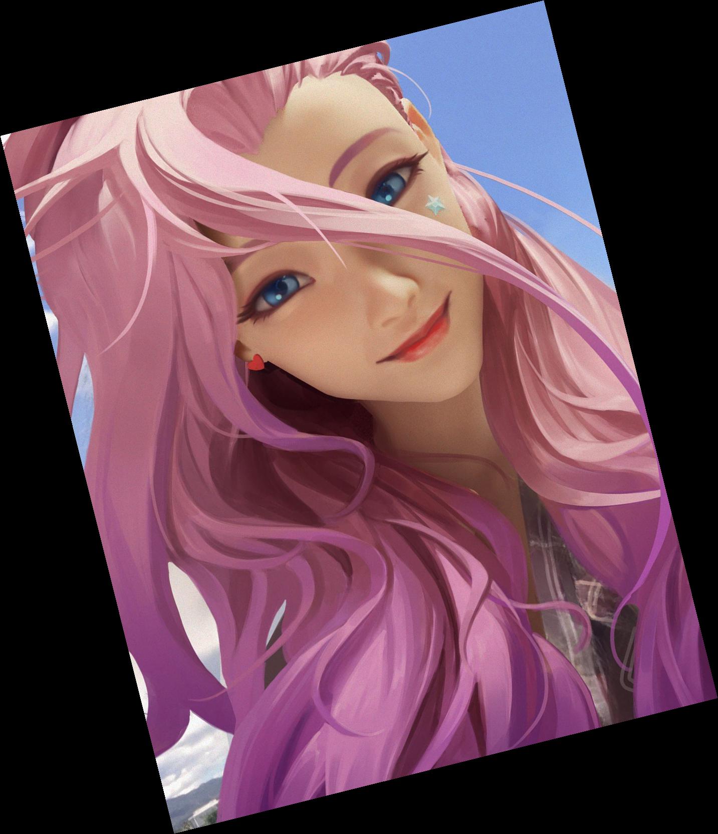
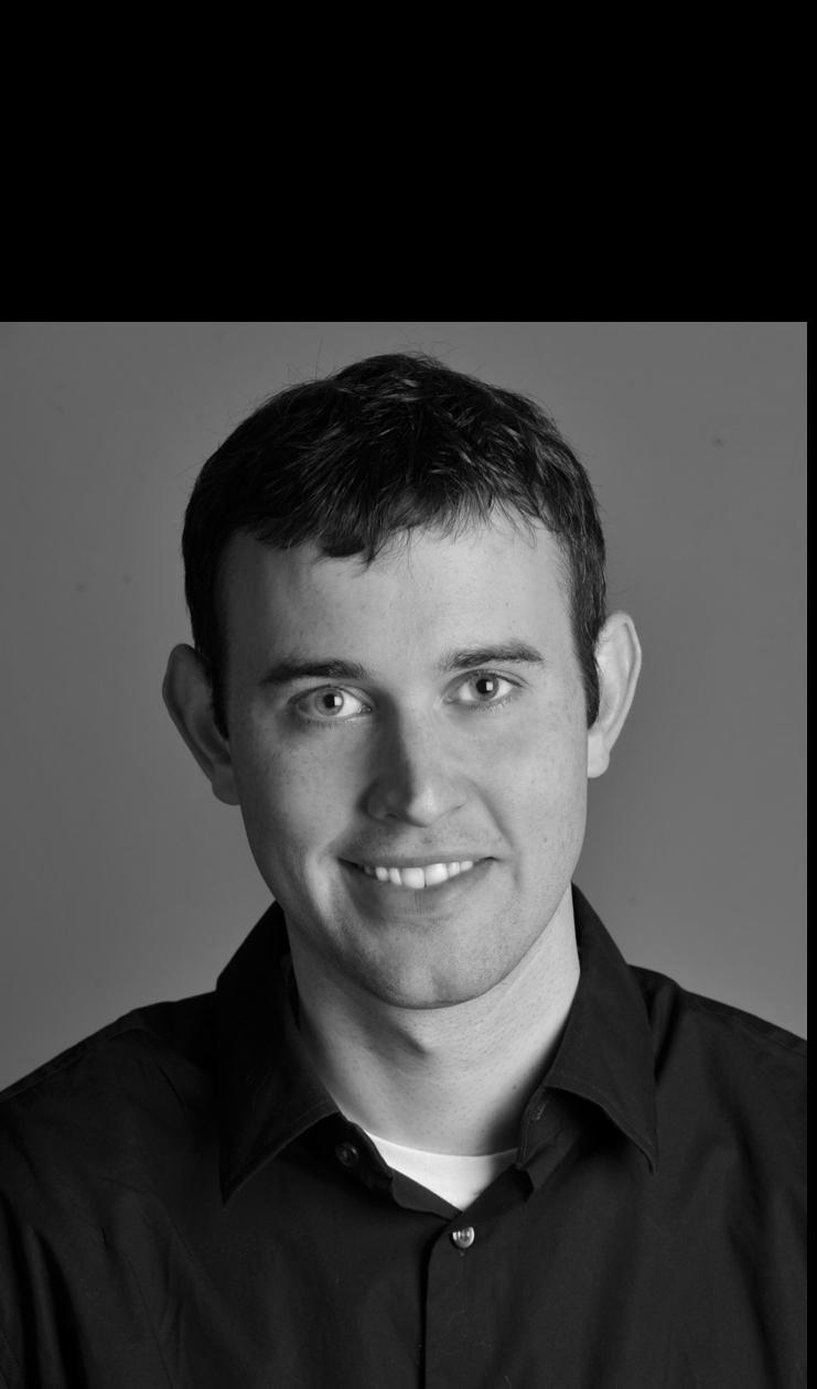
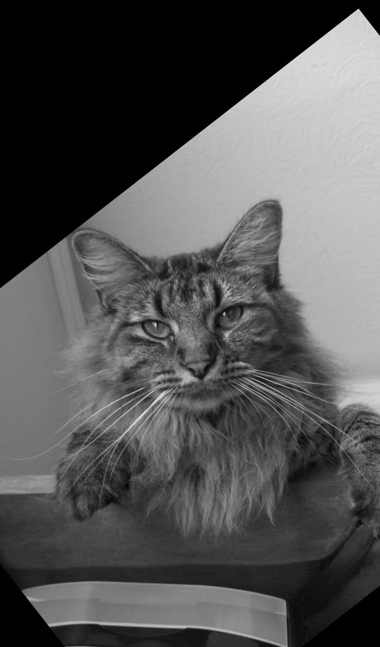
I expected the above lake image to fail, since there is a lot of reflection and different terrain going on, but it actually surprisingly worked very well! I found, however, that the below image is very difficult to align, presumably because of lack of horizon and dominating hair going in so many different directions (this difficulty is clear from the messier histogram as well).
Part 2: Fun with Frequencies!
Part 2.1: Image "Sharpening"
We attempt to sharpen images by creating a blurred version (by convolving with a Gaussian filter), subtracting these low frequency signals from the original to isolate the high frequency edges, and adding these back to the orignal image.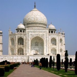
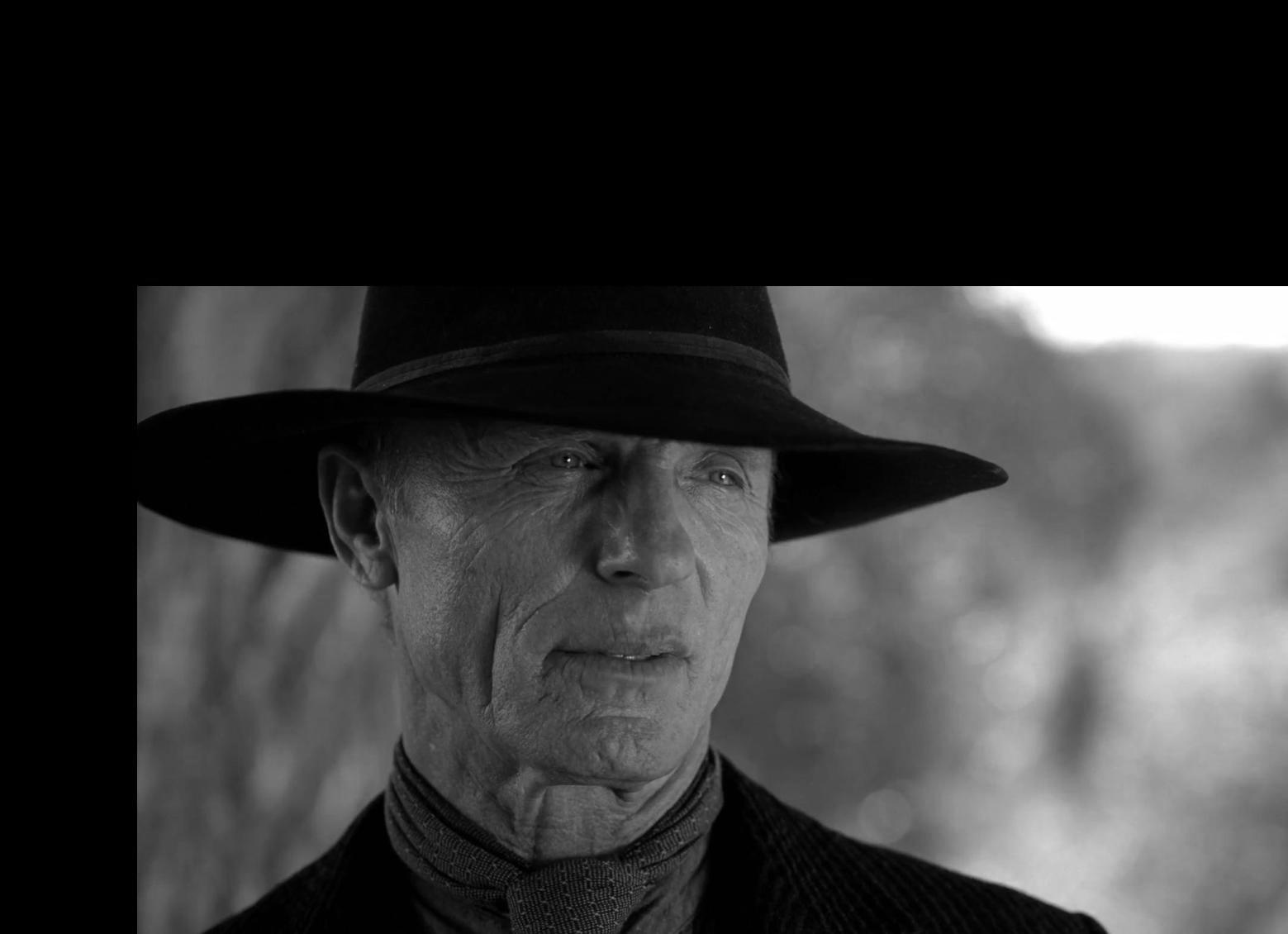
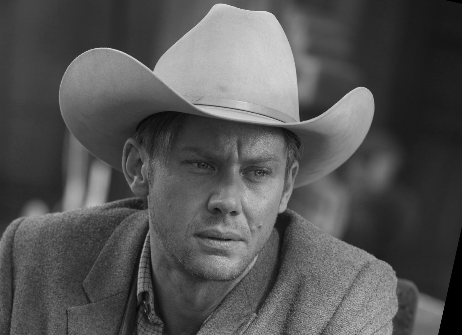
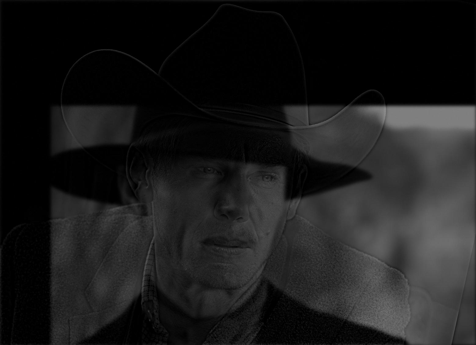
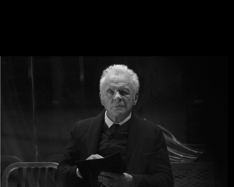
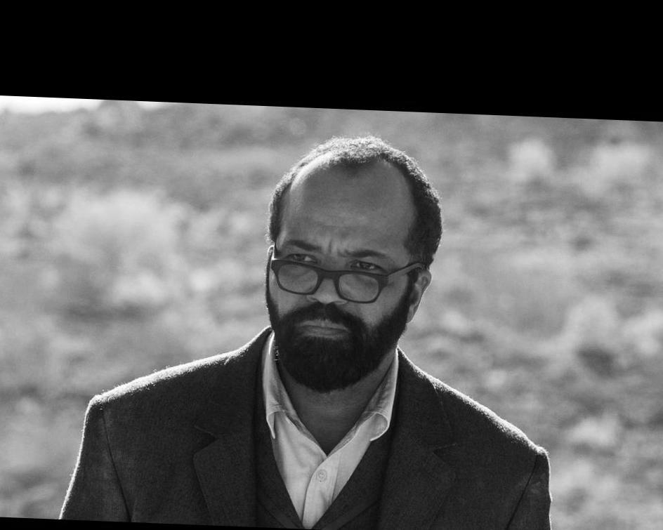
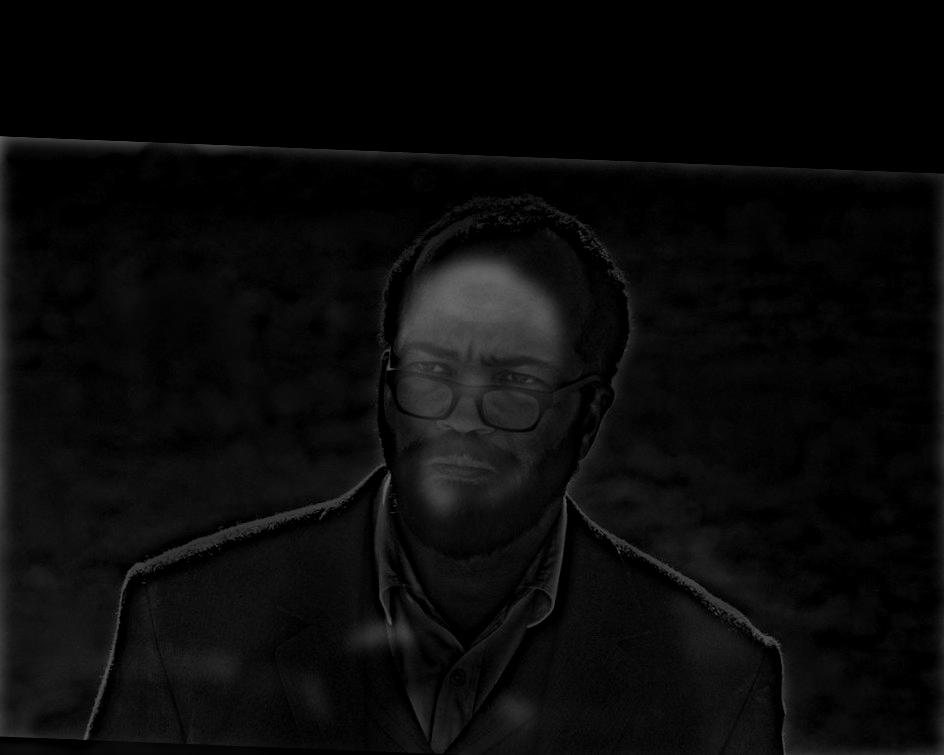
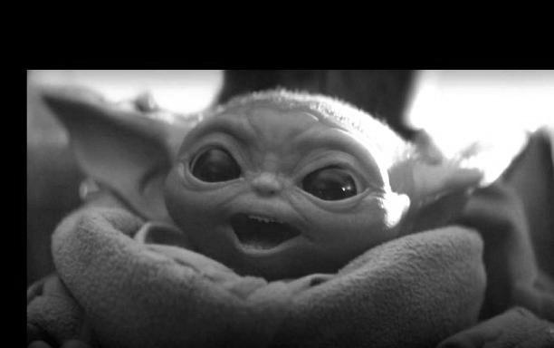
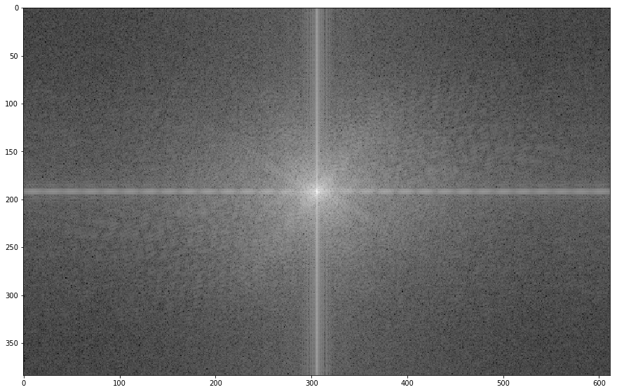
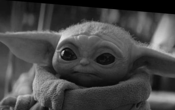
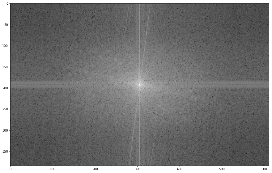
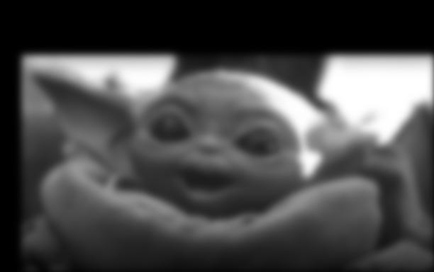
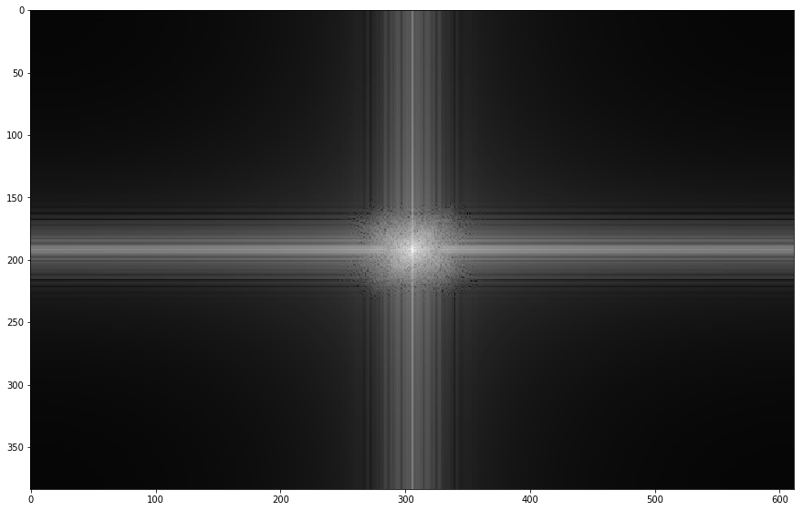
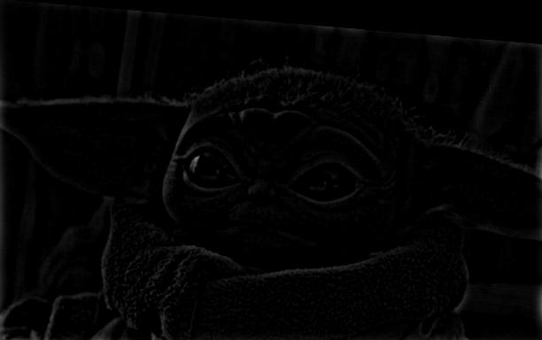
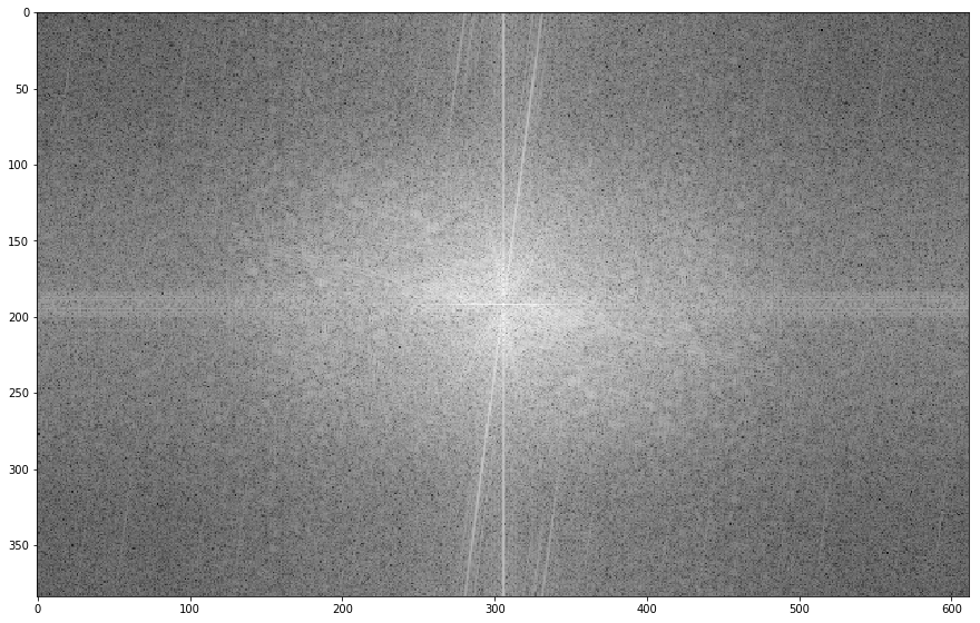
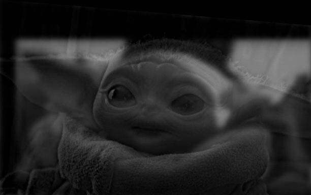
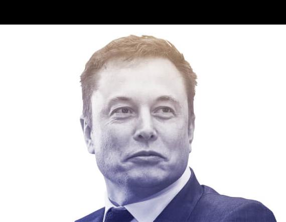
Part 2.2: Hybrid Images
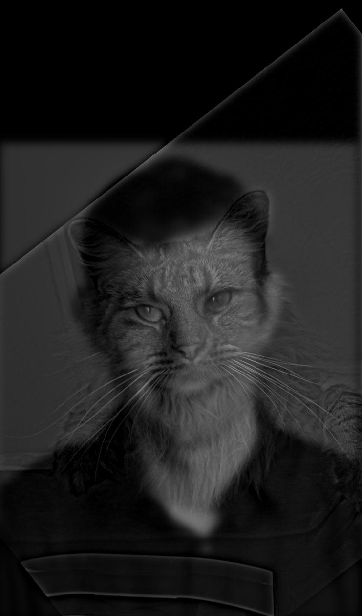
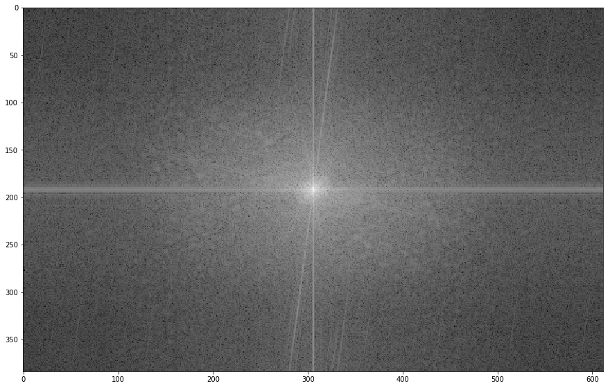
The following is a FAILURE CASE for hybrid images. This is primarily due do the difficulty in alignment and the vastly different objects and settings.
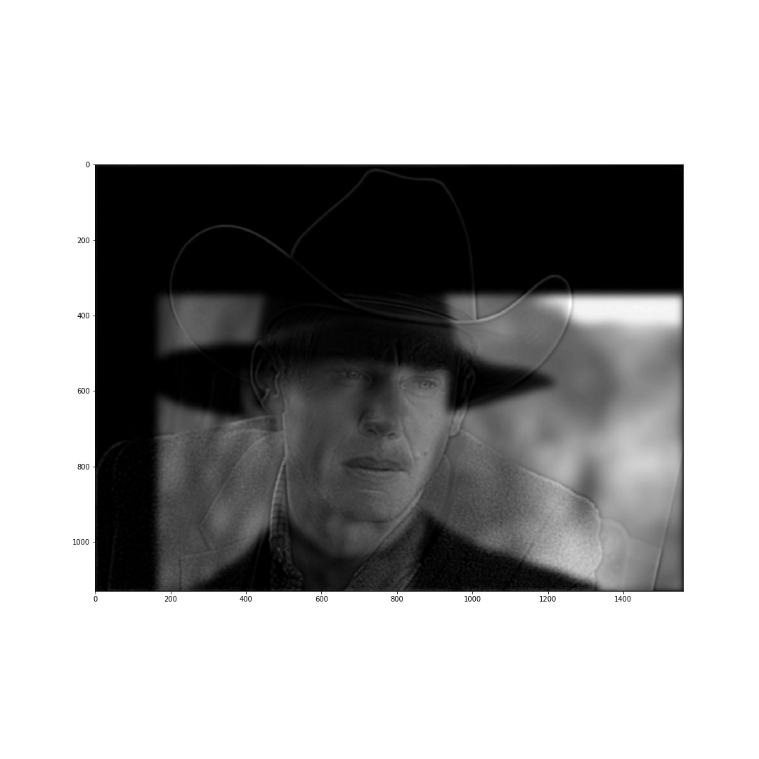
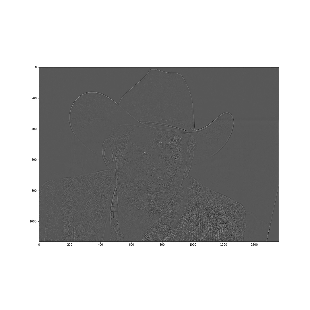
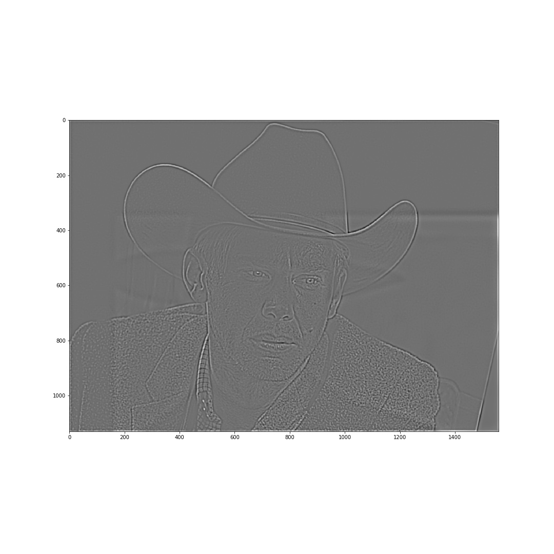
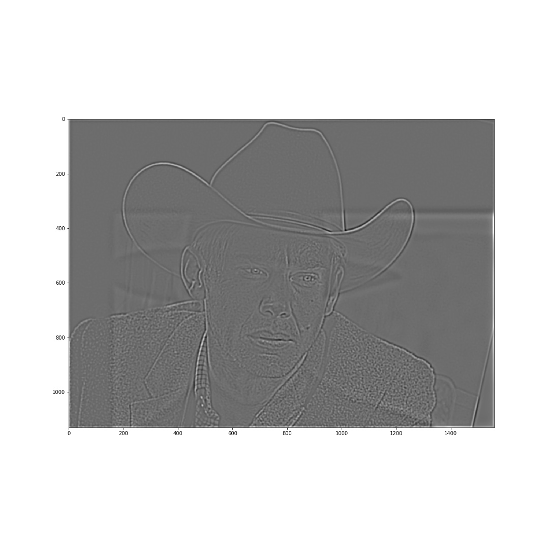
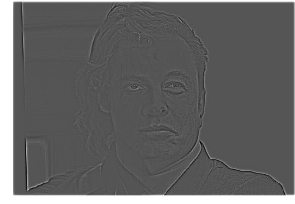
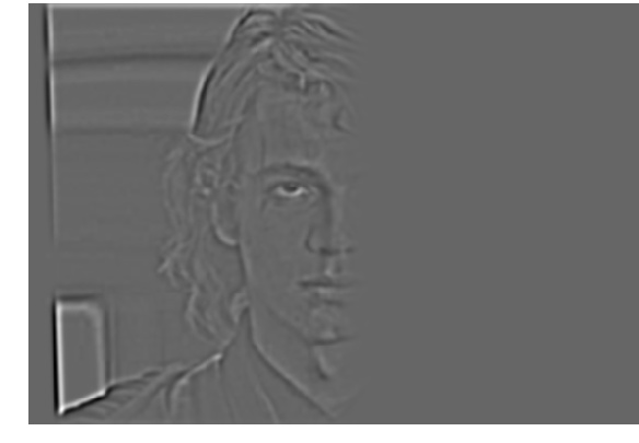
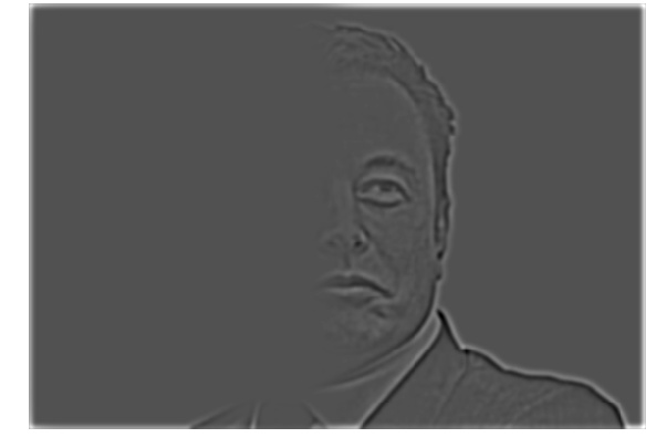
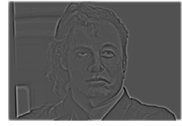
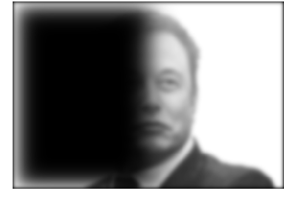
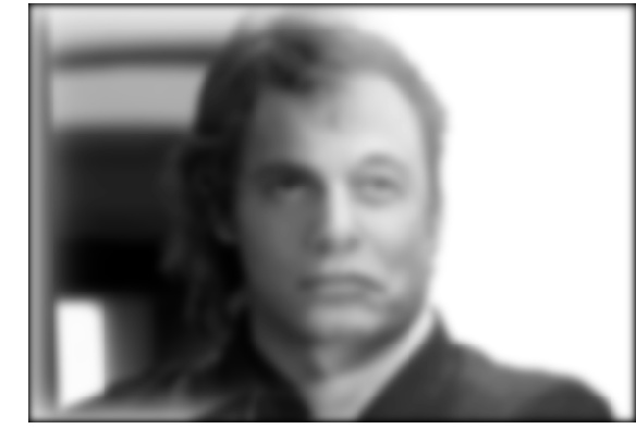
Part 2.3: Gaussian and Laplacian Stacks
Appliying Gaussian and Laplacian stacks to Salvador Dali's Lincoln and Gala.

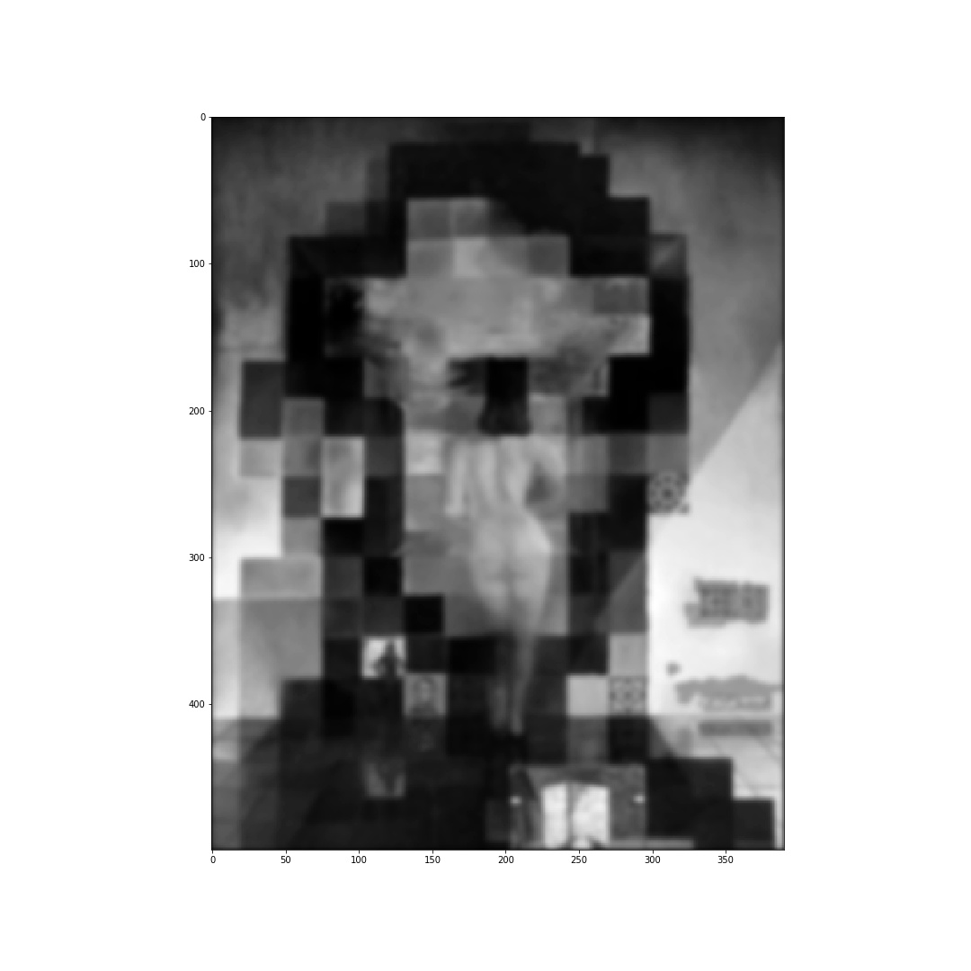


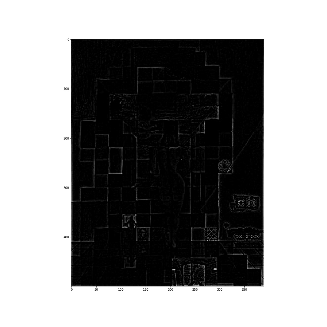
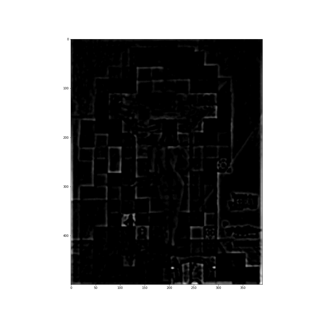


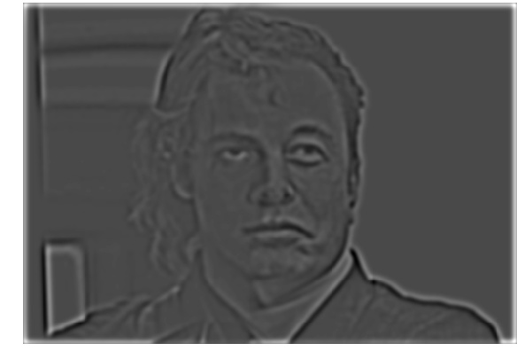
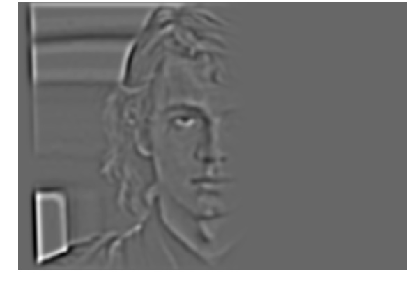
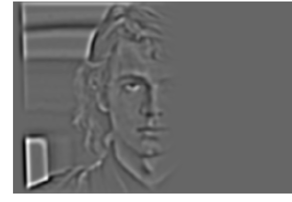
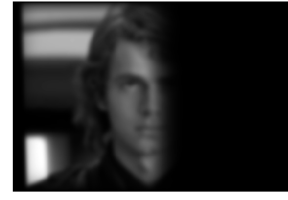
Appliying Gaussian and Laplacian stacks to Hybrid Image of old and young version of William, Gaussian stacks reveal low frequencies (old) while Laplacian stacks reveal high frequencies (young).


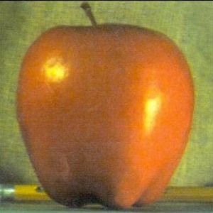
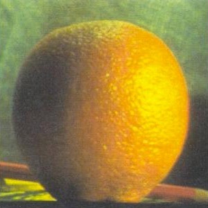
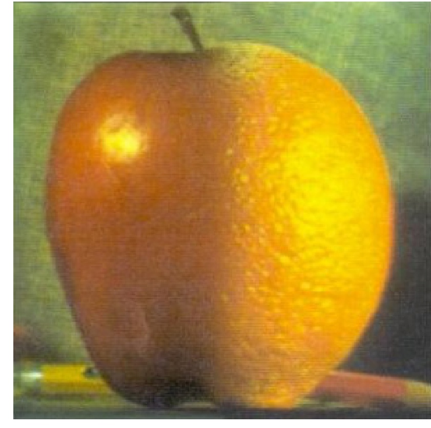
Part 2.4: Multiresolution Blending (a.k.a. the oraple!)
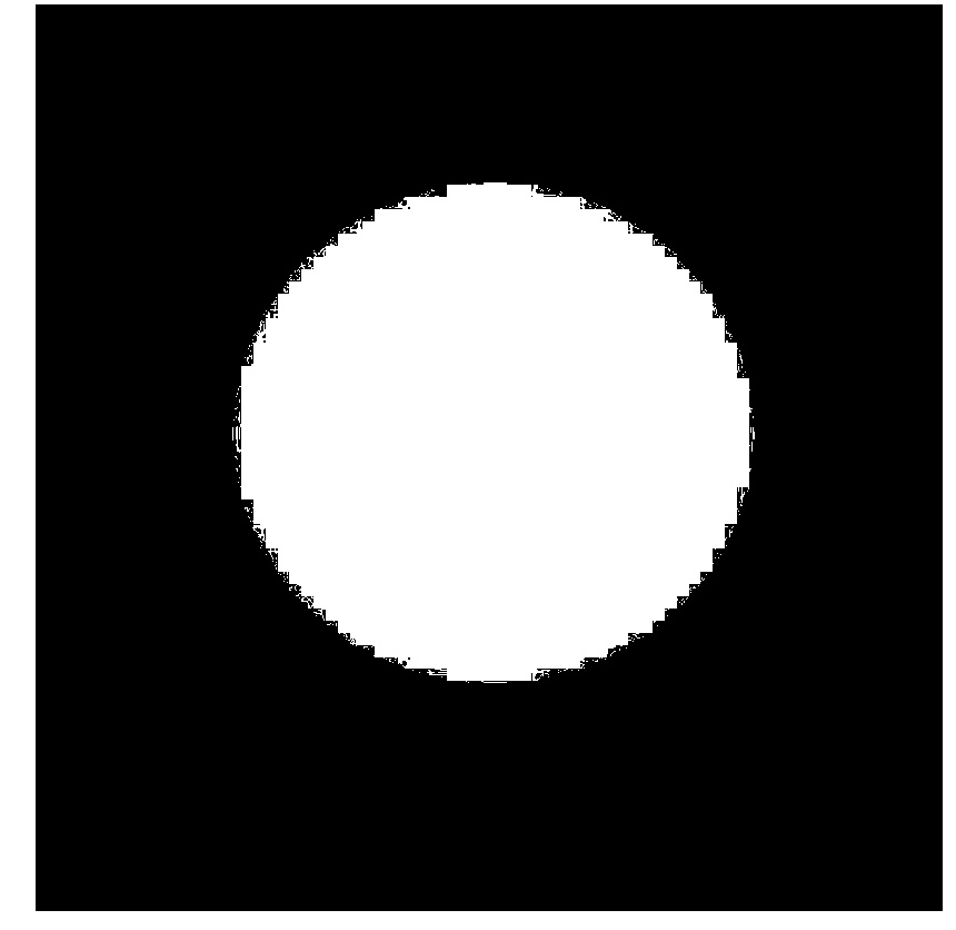
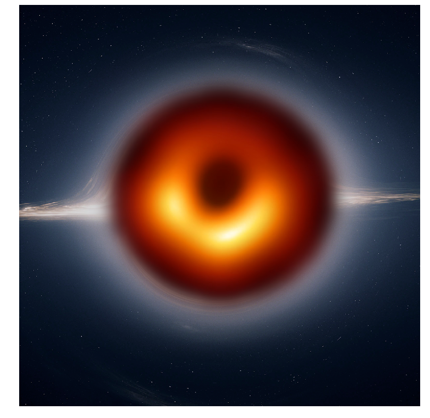
For this part we blend 2 images at multiple resolutions by adding their Laplacian stacks together, weighting elementwise with a Gaussian stack of a mask.
Bells and Whistles (adding color)
For the first 2 examples I used the standard horizontal mask, splitting image into 2 (left and right).
Apple + Orange
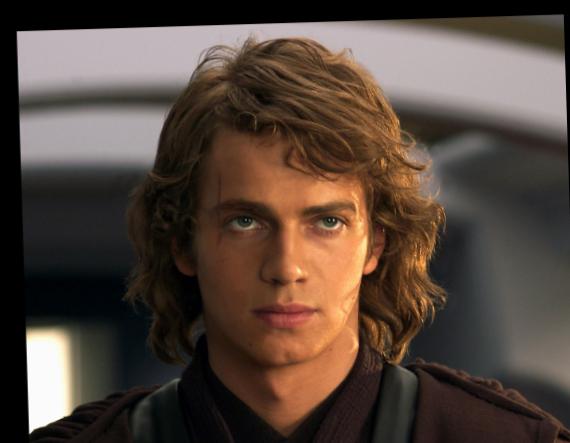
Anakin + Musk
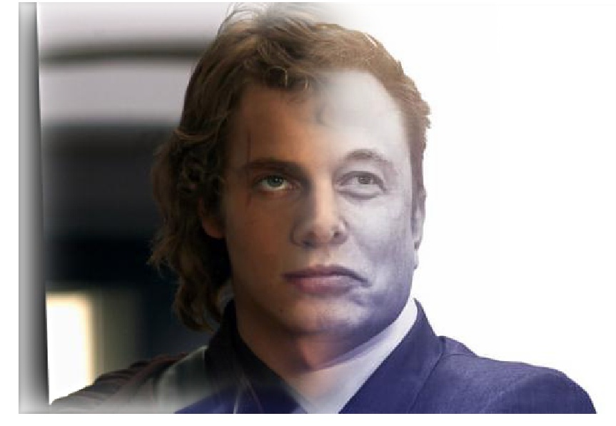
I also display the Laplacian stack and masked input images (for grayscale version) for each layer.


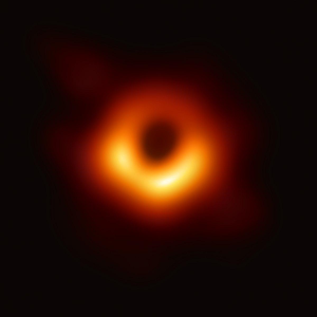
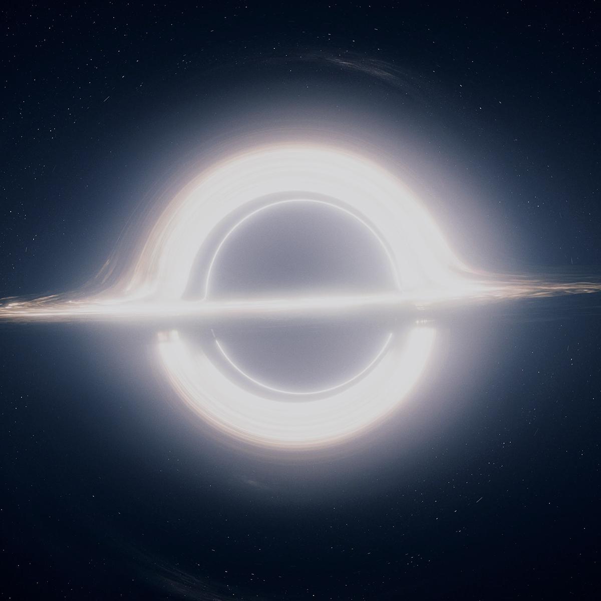
For the next part I drew an irregular mask (oval) to blend one black hole into the inside of another.