CS 194-26: Project 2
Akshit Annadi
1.1
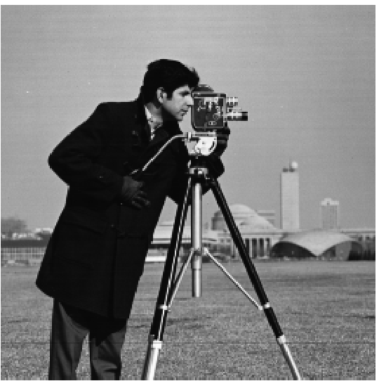
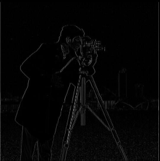
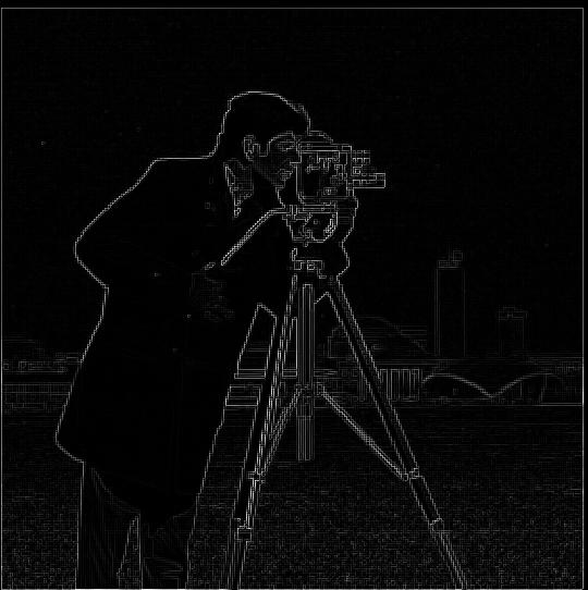
In this portion of the project, we analyzed the edges in the following image of a cameraman.
To get an edge image, we first got the partial derivative in x of the image by convolving it with the filter [[1,-1]]. Similarly
we got the partial derivative in y of the image by convolving it with [[1],[-1]]. These images are pictured below.
We used the partial derivative images to get the gradient magnitude image by using the following formula: magnitude = sqrt(dx^2 + dy^2). After computing the gradient
image which is pictured below, I expirementally found a threshold(.18) such that all pixels above that threshold would be considered part of an edge and all below would not.
The resulting edge image is shown below.
X Gradient
Y Gradient
Gradient Magnitude
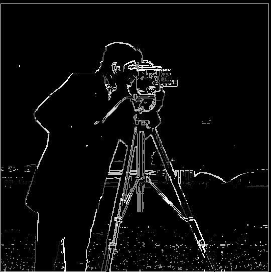
Binarized Edge Image
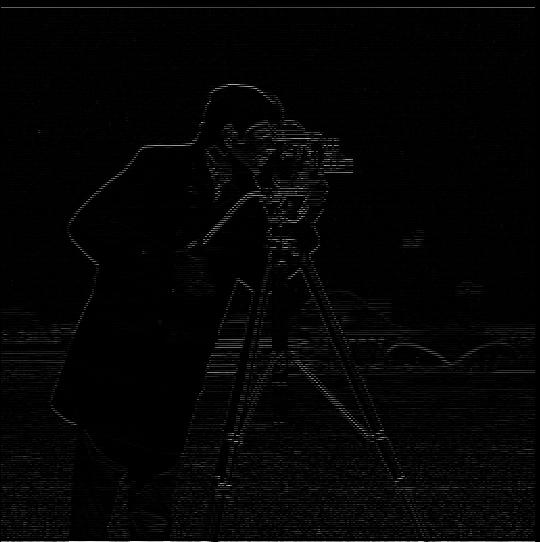
1.2
In part 1.1, the resulting edge image had a lot of noise, particulary in the grass at the bottom. To alleviate this problem, we used a guassian filter(8x8, sigma=2)
to smooth the image. After smoothing the image, I ran the same process as 1.1 to produce an edge image with a threshold of .03, pictured below. The main differences are that there is much
less noise from the grass, which is due to the fact that the grass was "smoothed" out, and that the edges are thicker due to the fact that the gaussian filter made the pixels surrounding the true
edges inherit some of the values from the edges.
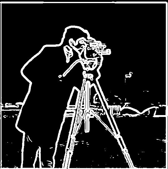
Binarized edge image with 2 filters
Instead of running the guassian filter and then the derivative filters on the image seperately, we could convolve the guassian with the derivative filters and do one set of convolutions on the
image due to the associative property of convolutions. This ended up, as expected, producing the same result. The derivative of guassian filters and the resulting edge image are shown below.

dx Gaussian Filter

dy guassian filter

Binarized Edge Image
1.3
In this part of the project, we used the gradient and edge detection methods from the previous parts to make a program that automatically straightens images. It does this by
computing the number of vertical and horizontal edges in an image over a set of proposed regions and choosing the rotation that results in the maximum amount of horizontal/vertical edges.
The number is computed by doing the following for each image:
- Rotate the image by the proposed rotation
- Crop a specified amount from each side of the rotated image to ignore the edges created by the rotation itself
- Compute the gradient magnitude image as specified in 1.2
- For each pixel that has a gradient value greater than a specified amount, get the derivative at that pixel in the x and y directions and compute the angle of the edge using the following formula: angle = arctan(dy/dx)
- Compile a list of such angles and count the number of ones that are approximately 180, 90, 0, -90, and -180
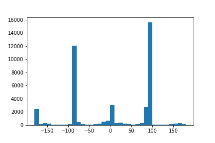
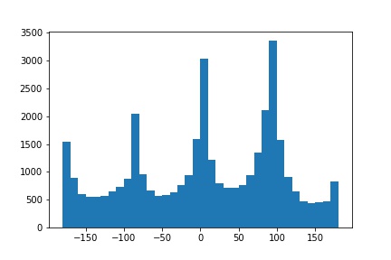
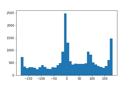
A total of 10 angles were tried for each image, ranging from -10 to 10 degrees. The result of running this algorithm is shown on three images below along with a histogram of the angles for both the straightened and original versions of the images. Note that since the angle of rotation was typically less than
5, a large change in the histogram bins is not really visible.
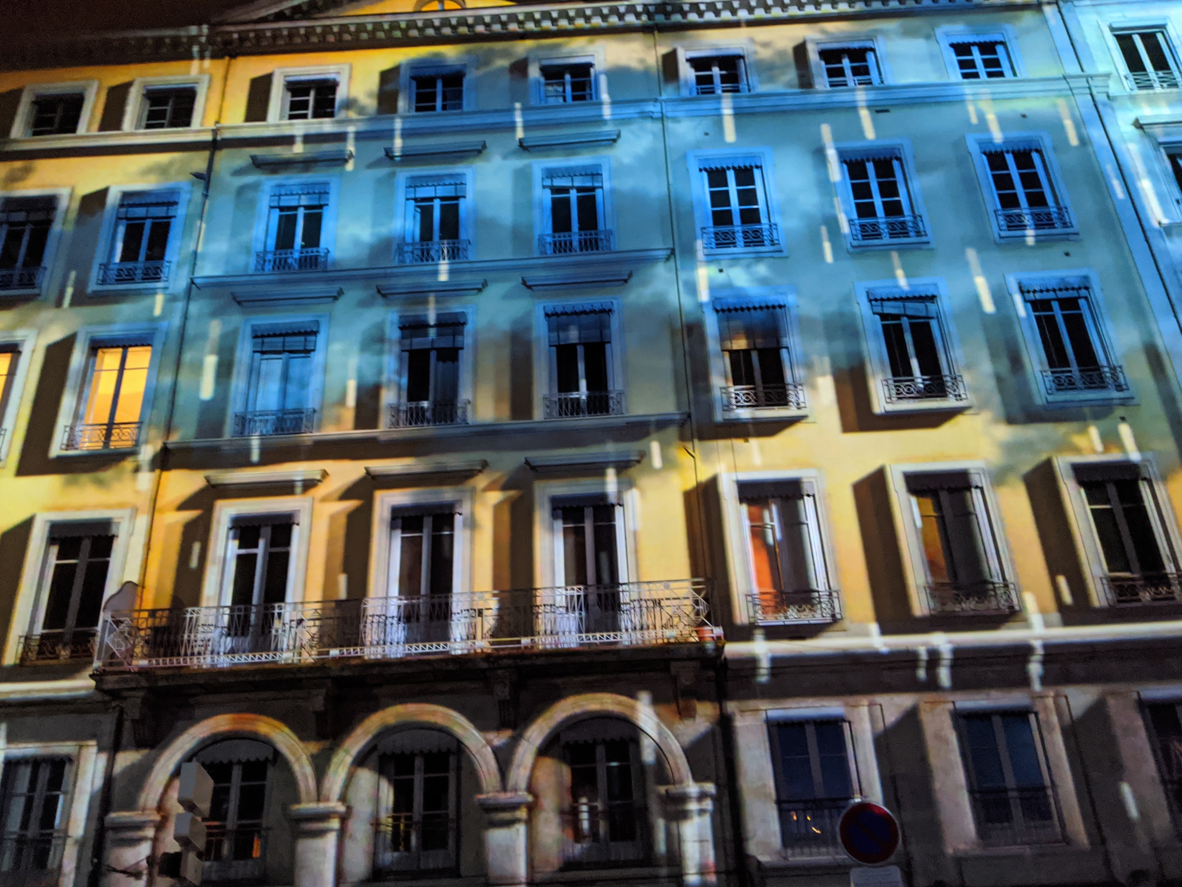
facade
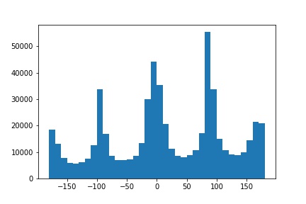
facade angle histogram
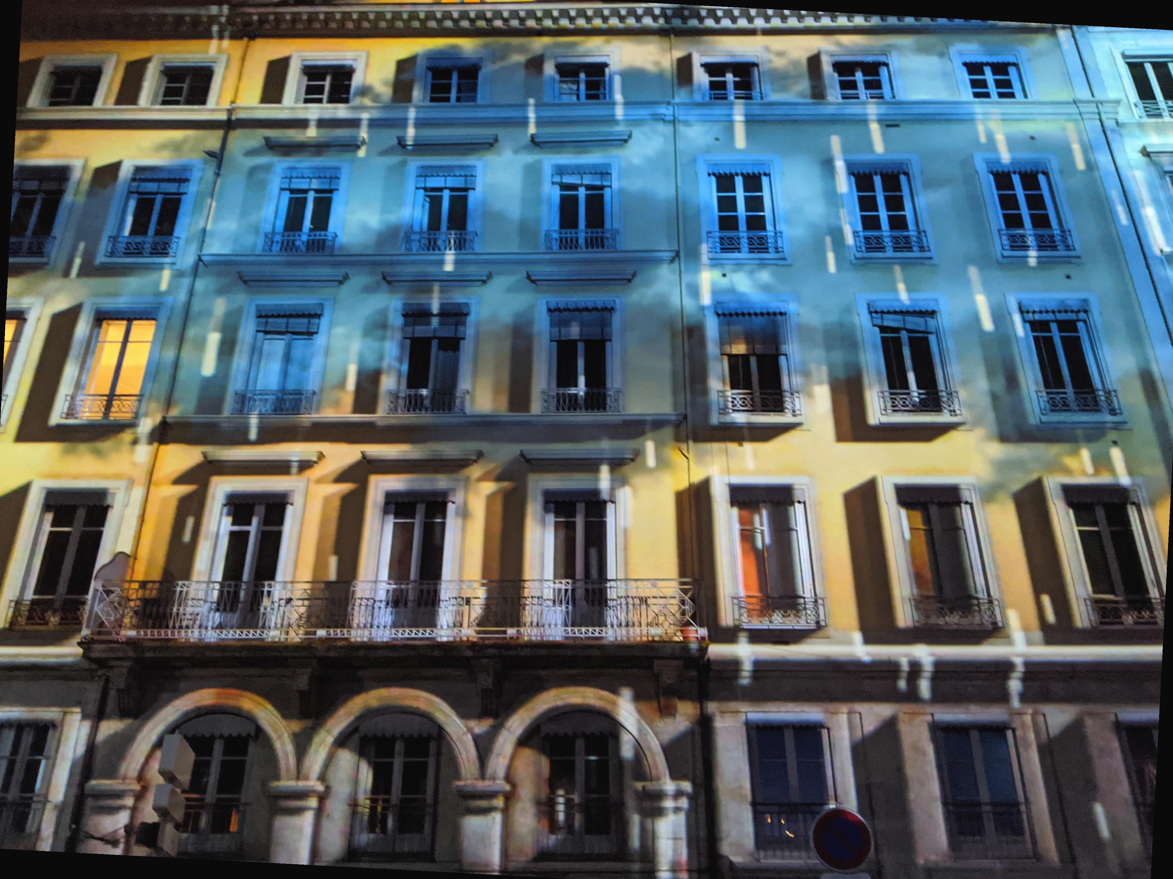
straightened facade
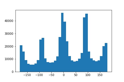
straightened facade histogram
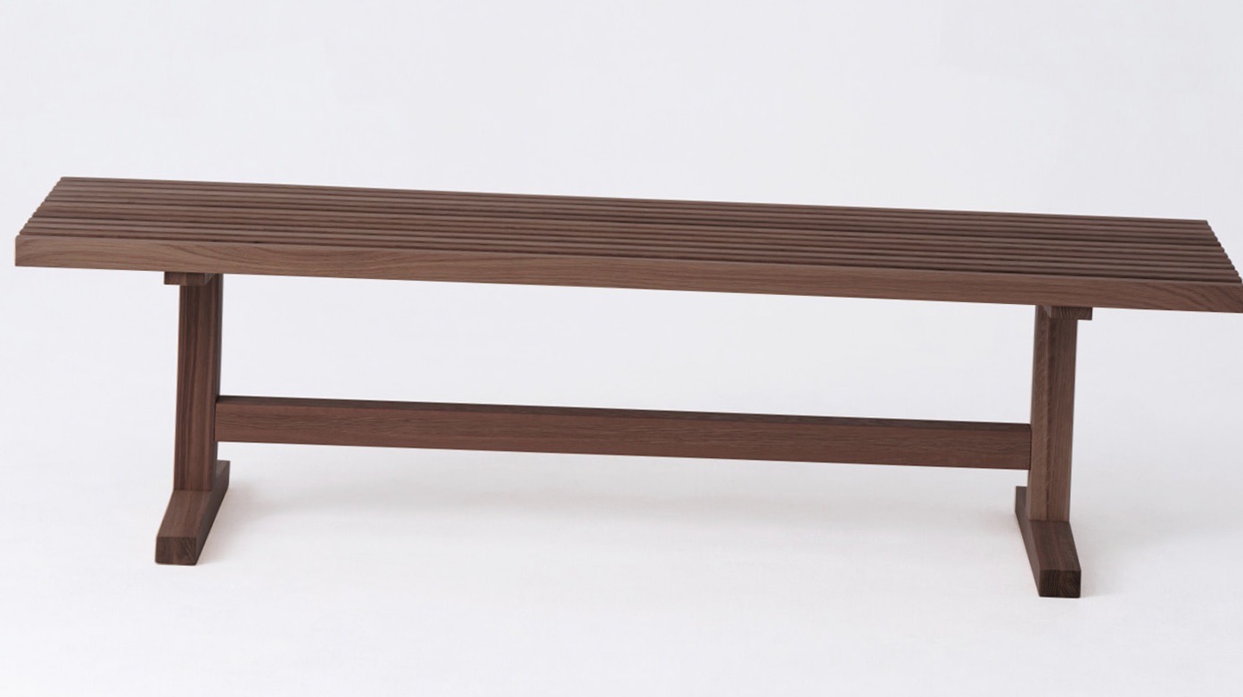
bench
bench angle histogram
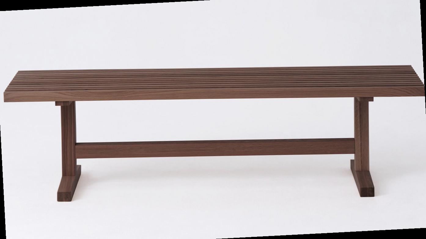
straightened bench
straightened bench histogram
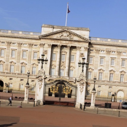
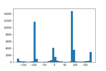
buckingham
buck angle histogram
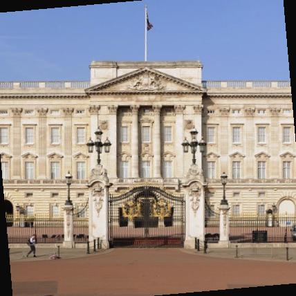
straightened buck
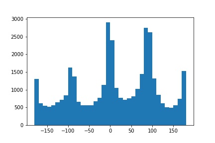
straightened buck histogram
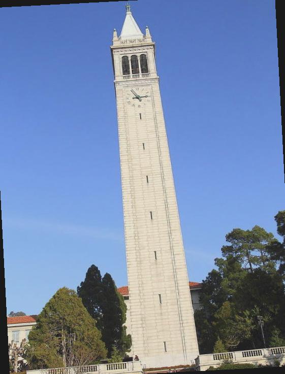
Failure Case
The following is a case where the algorithm failed to straighten an image. This is due to the fact that there are a lot of extraneous edges caused by the tree and other objects that aren't
vertical or horizontal in the actual straight version of the image.
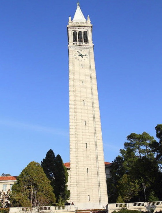
campanile
campanile angle histogram
straightened campanile
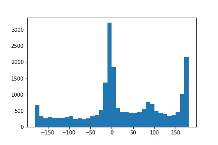
straightened campanile histogram
2.1
In this part of the project, we used guassian filters to sharpen images. This was done by filtering the image with a guassian as a low pass filter and subtracting the result from the original image
to isolate the high frequencies in the image. The high frequencies were multiplied by an alpha value and added back to the original image to create the sharpened image.
All these operations can be combined into a single convolution operation where the image is convolved with the following filter: (1 + alpha) * e - g * alpha, where e is the unit impulse filter
and g is a guassian filter. The following images were sharpened using a guassian of size 20 with sigma 4 and an alpha value of 1.
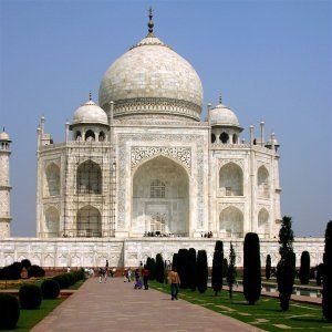
taj.jpg
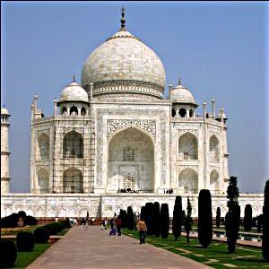
sharpened taj
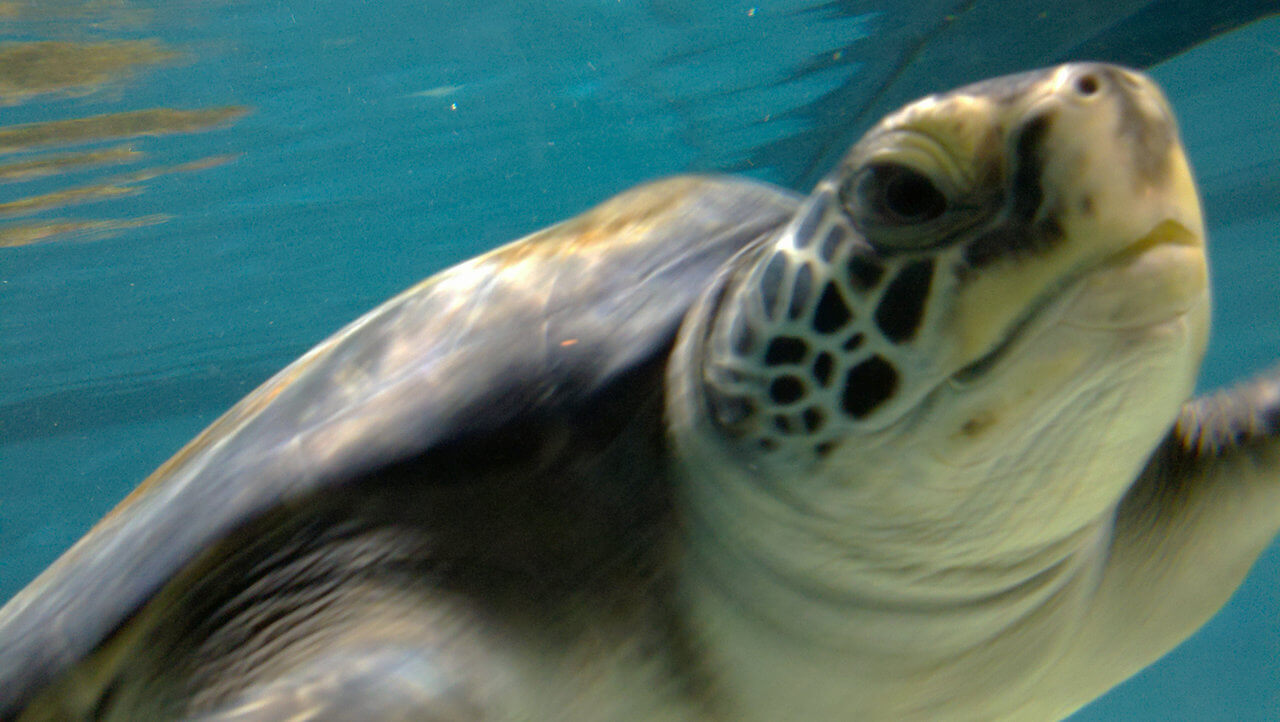
turtle.jpg
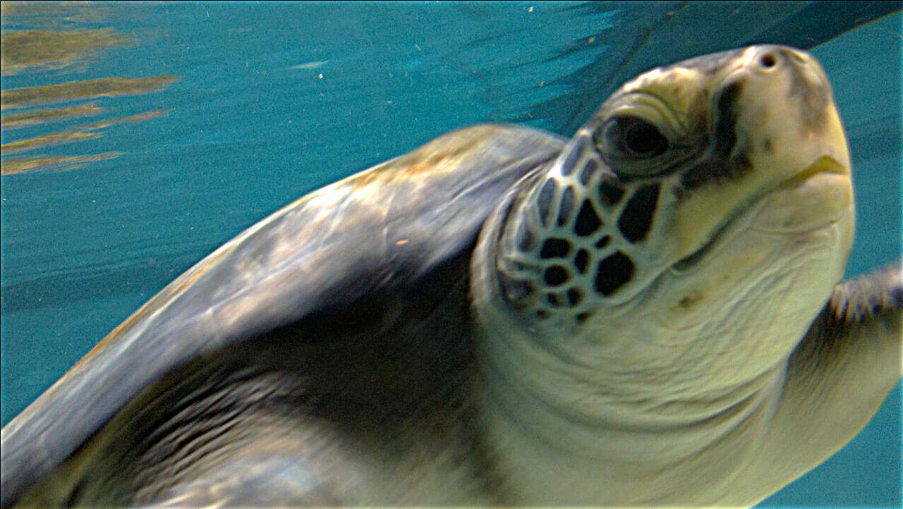
sharpened turtle
Blur then Sharpen
The following is a case where a clear image was taken, blurred using a guassian filter, then sharpened using the algorithm above. Note that while the sharpened image is more defined than
the blurred one, it still is not identical to the original, as the high frequencies of the original were lost when blurred.
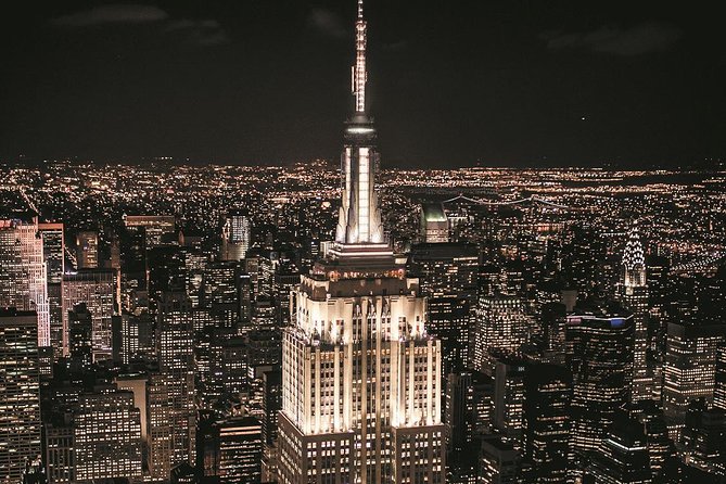
city
blurred city
sharpened city
2.2
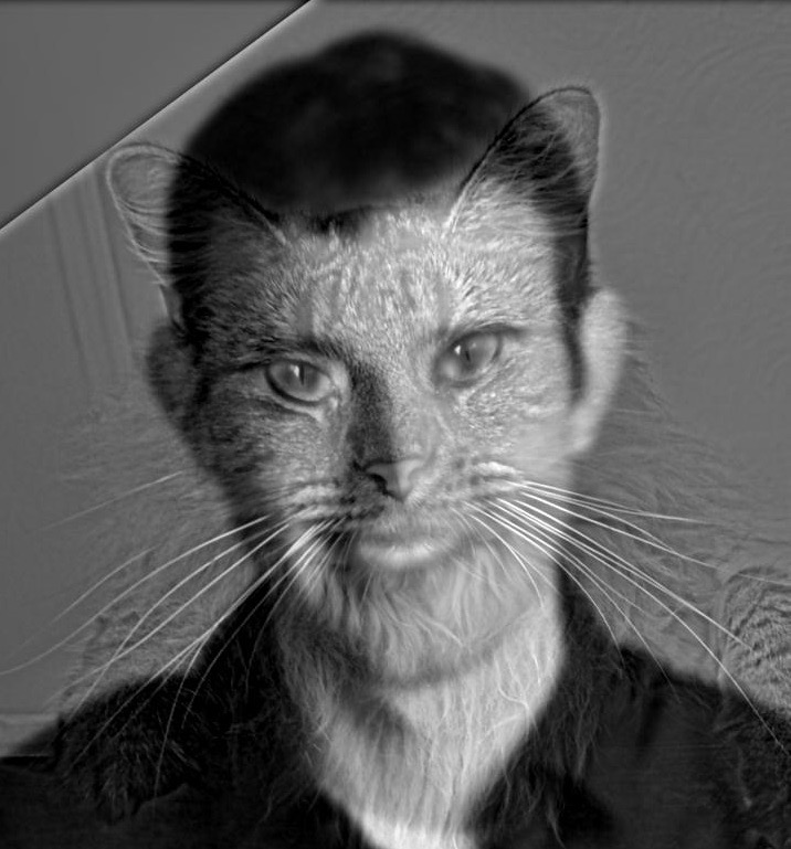
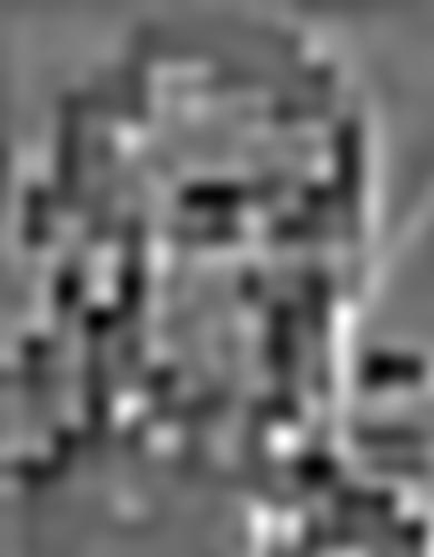
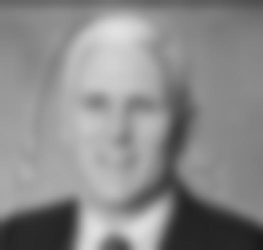
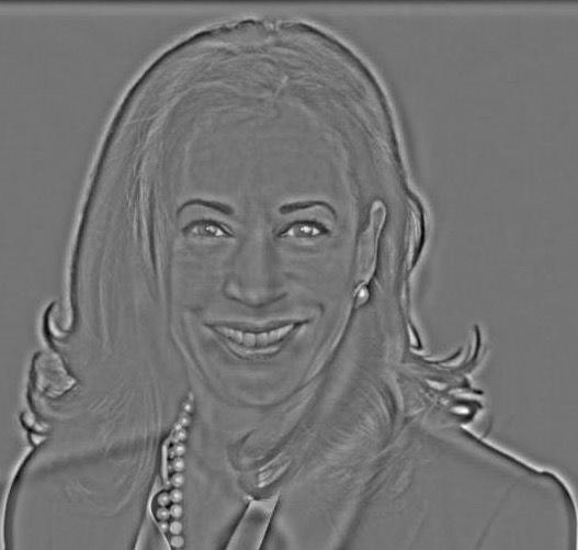
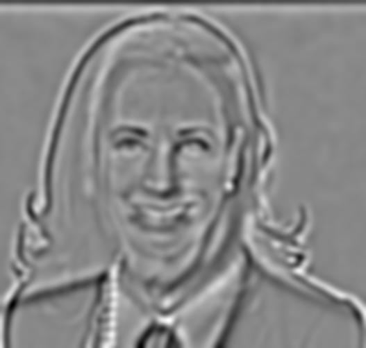
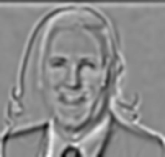
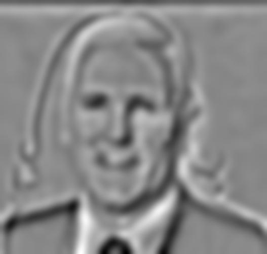
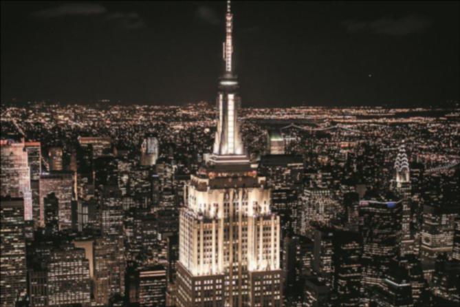
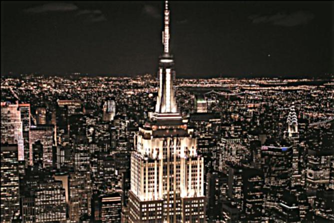
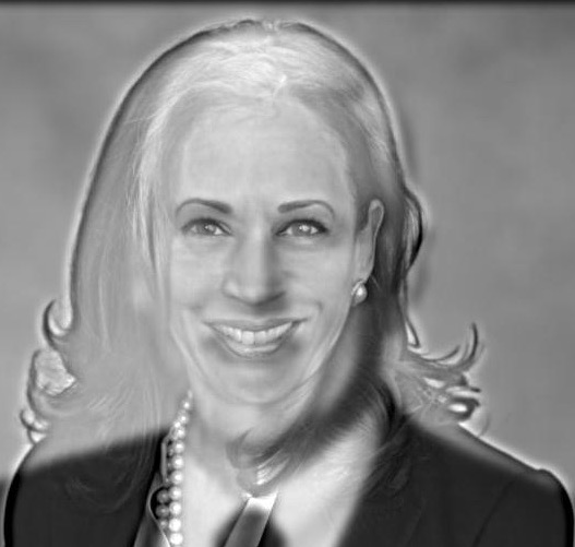
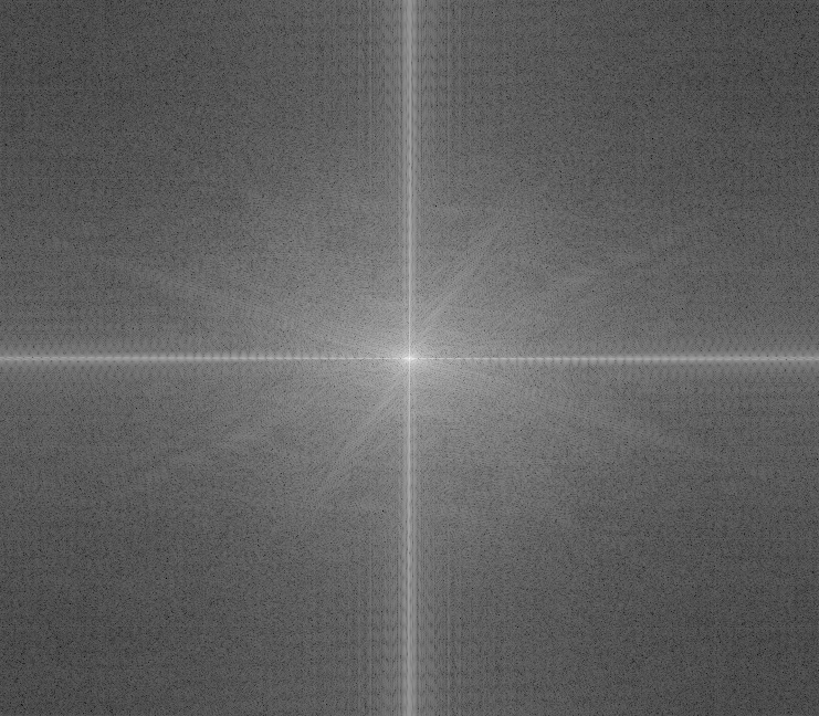
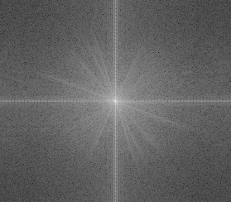
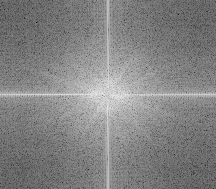
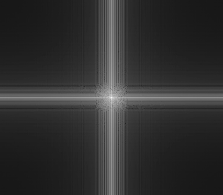
In this part of the project, we created "hybrid images" that would change in interpretation as a function of the viewing distance. First the images were aligned using code provided to us. After this, I isolated the high frequencies of the image on the left
and the low frequencies of the image on the right using guassian filters(20x20 with sigma=8 for high pass and 20x20 with sigma=5 for low pass) and combined them to create the result. At close distances, the high frequencies dominate and one picture is visible.
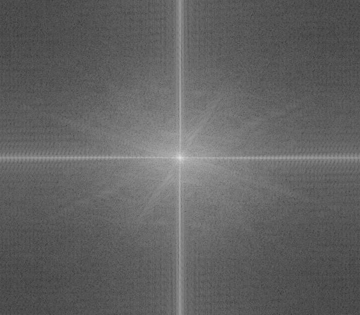
At far distances, the low frequencies are most visible and the other picture is visible. A fourier analysis of the first example is also displayed, showing the results of
the low/high pass filters on the images and the resulting hybrid in the frequency domain.
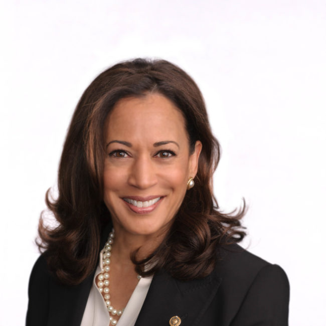
harris

pence
hybrid(big and small)
harris
pence
high pass harris
low pass pence
hybrid
Failure Case
The following is a case where the algorithm failed to create a hybrid image. This was due to the fact that the shapes in each of the images were so different to begin with and that they don't overlap, so both images are visible at close and far distances in the hybrid.
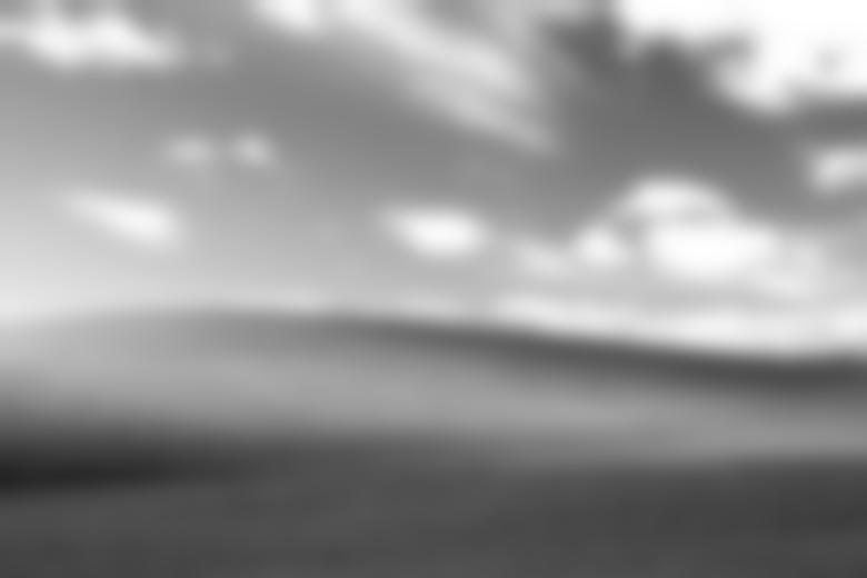
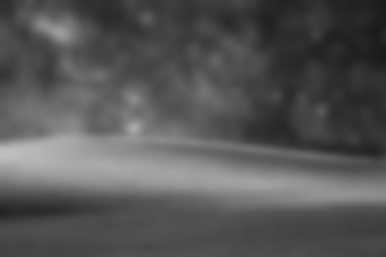
2.3
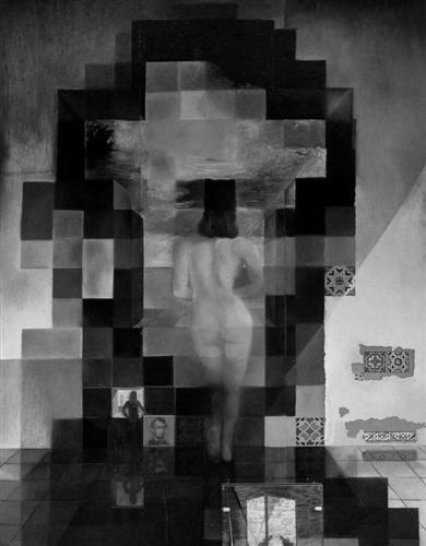
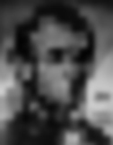
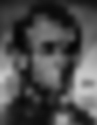
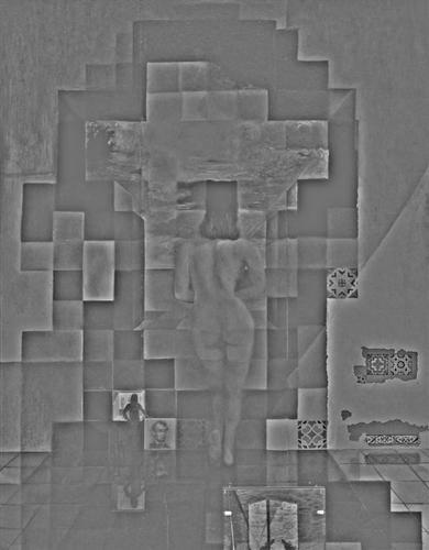
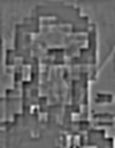
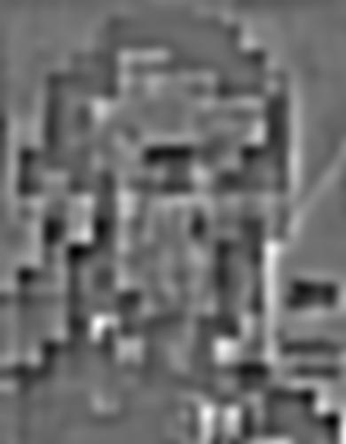
In this part of the project, I implemented Guassian and Laplacian stacks. To generate the Guassian stack for an image, I repeatedly applied a Gaussian filter(40x40, sigma=5) to the
image to create the levels of the stack. To create the levels of the Laplacian stack, I simply took the difference of each successive pair of levels in the Gaussian stack. The stacks for the lincoln image
and an image from the hybrid images above are shown below, with the Guassian stack in the top row and the Laplacian stack in the bottom row. The original images are the ones in the top left.
2.4
In this part of the project, the goal was to create a program that blended two images seamlessly. Merging two images just by cutting them together can produce
an ugly seam like the following:
stiched together without blending
However, the program I implemented produced a more gentle seam between images A and B with a mask M by using the following steps:
- Build Laplacian pyramids LA and LB for images A and B respectively.
- Build a Gaussian pyramid GM for the mask M
- Form a combined pyramid LS from LA and LB using nodes of GM as
weights. That is, for each level: LS(level) = LA(level)GM(level) + LB(level)*(1-GM(level))
- Obtain the splined image S by summing the levels of LS
The stacks were created using a filter of size 40 with sigma=3. The results on a few pairs of images are displayed below.
blended
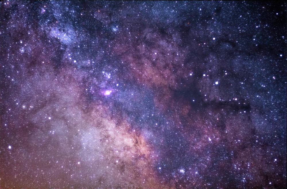
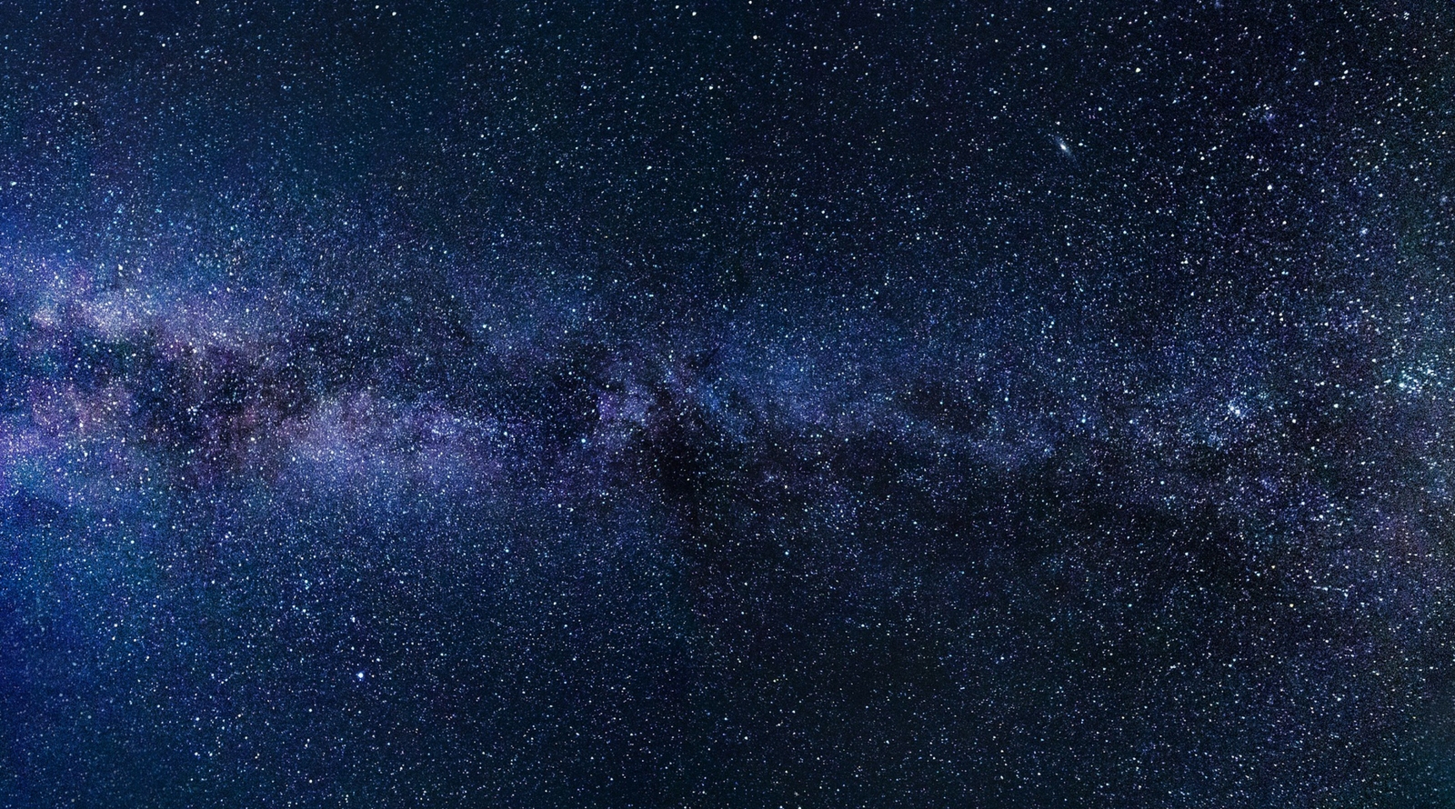
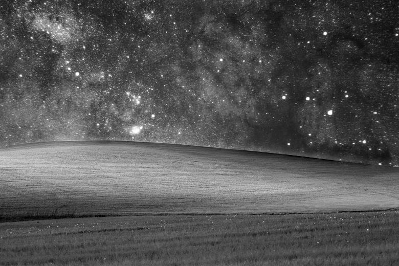
space
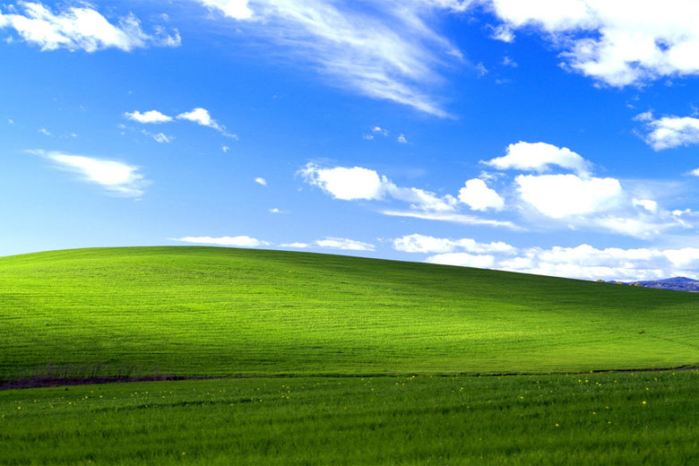
windows screensaver

mask
blended

stiched together without blending
the seam is a lot more abrupt
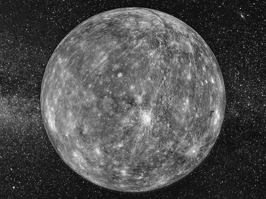
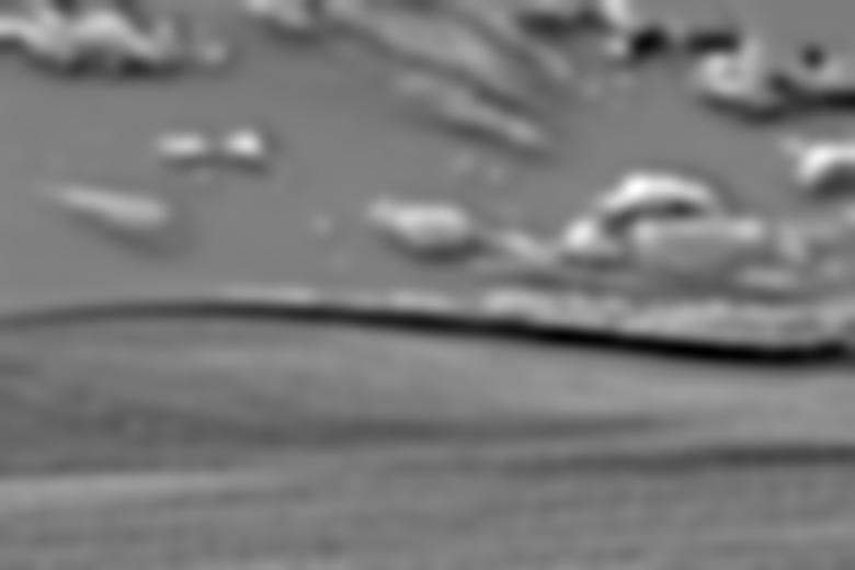
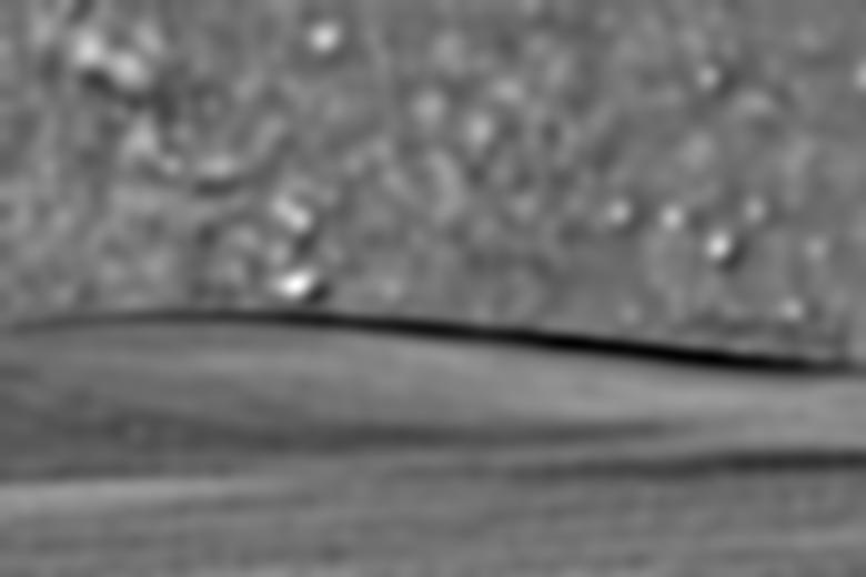
blended
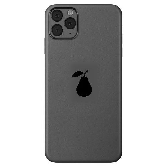
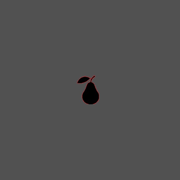
pearphone
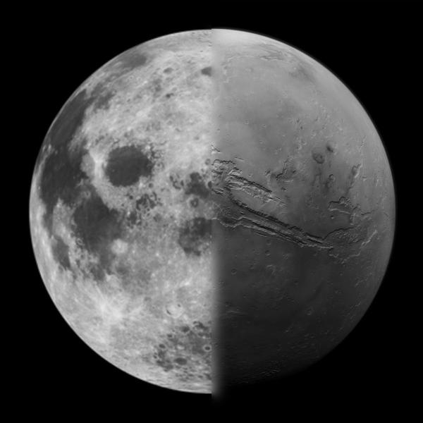
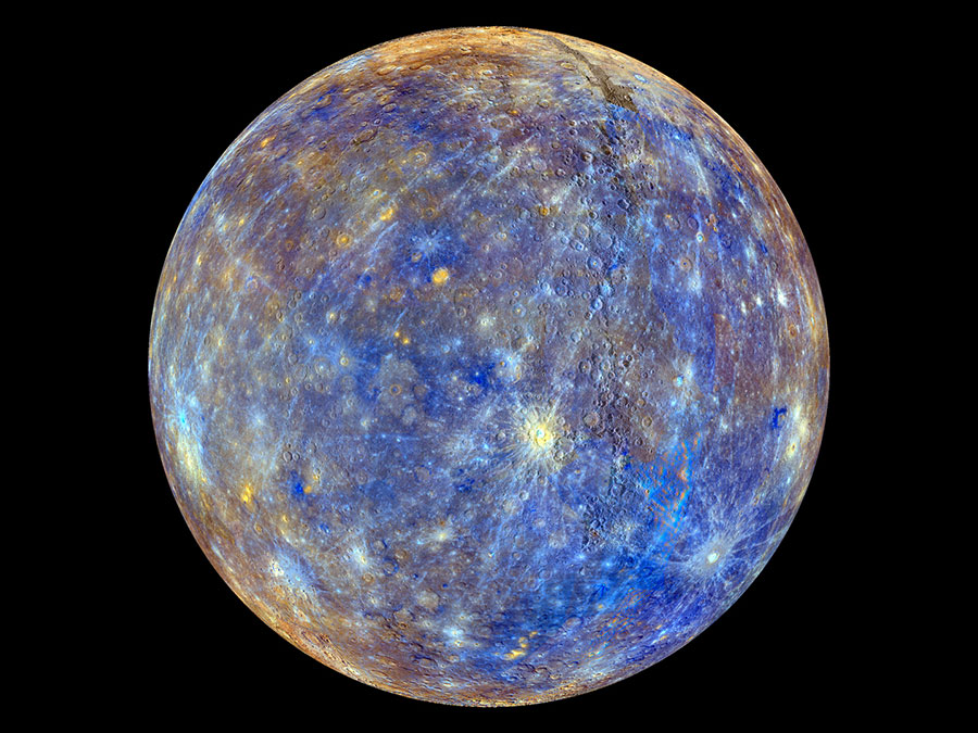
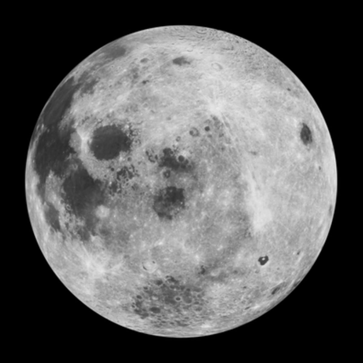
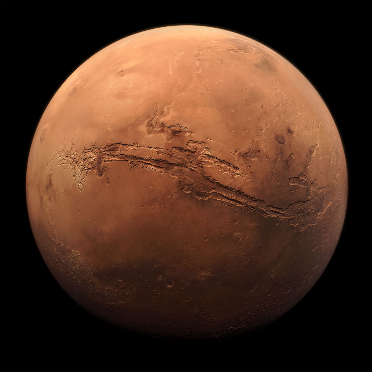
moon mars
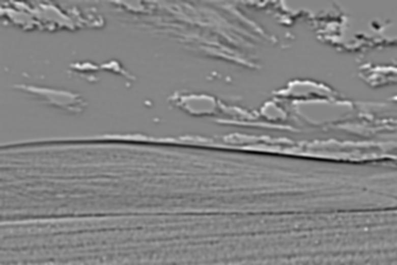
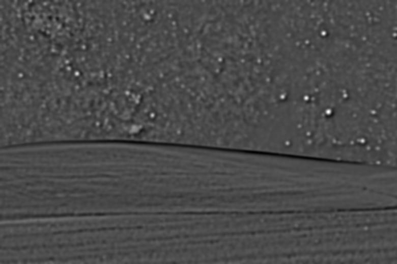
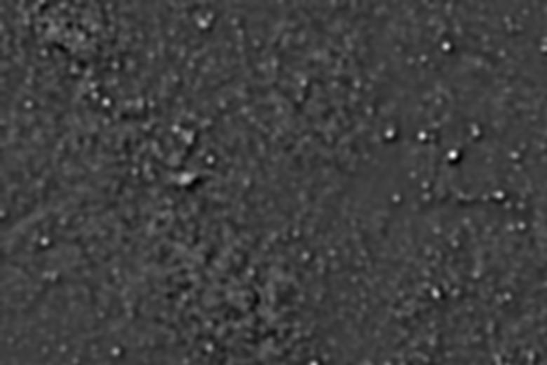
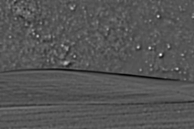
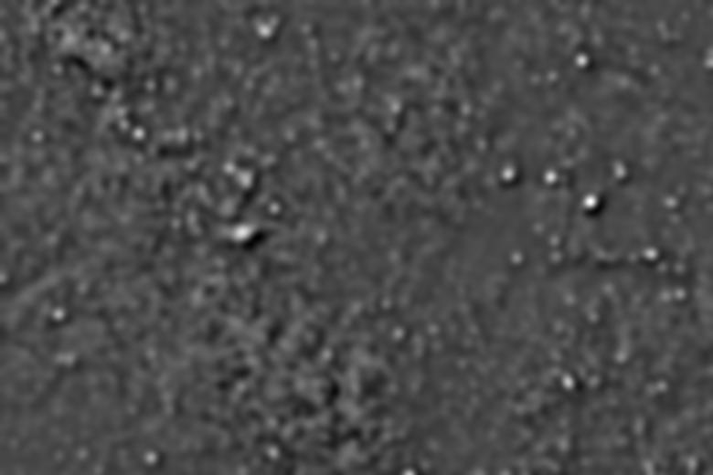
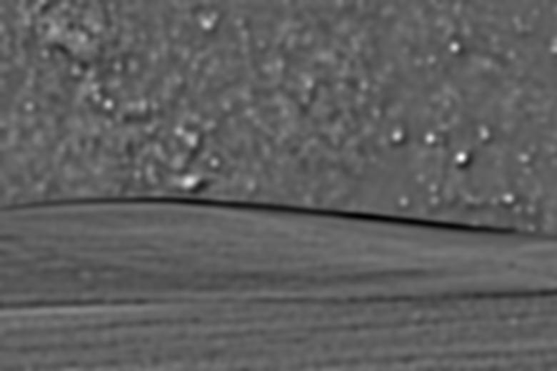
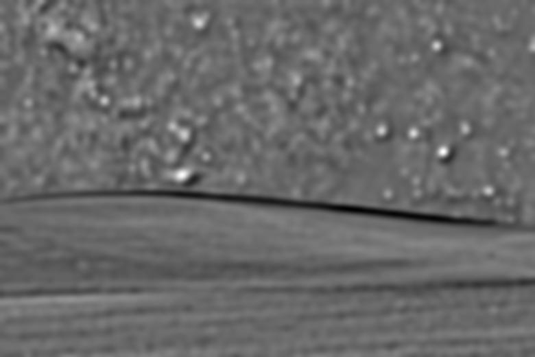
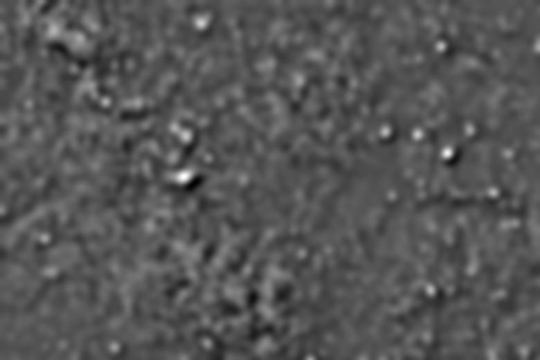
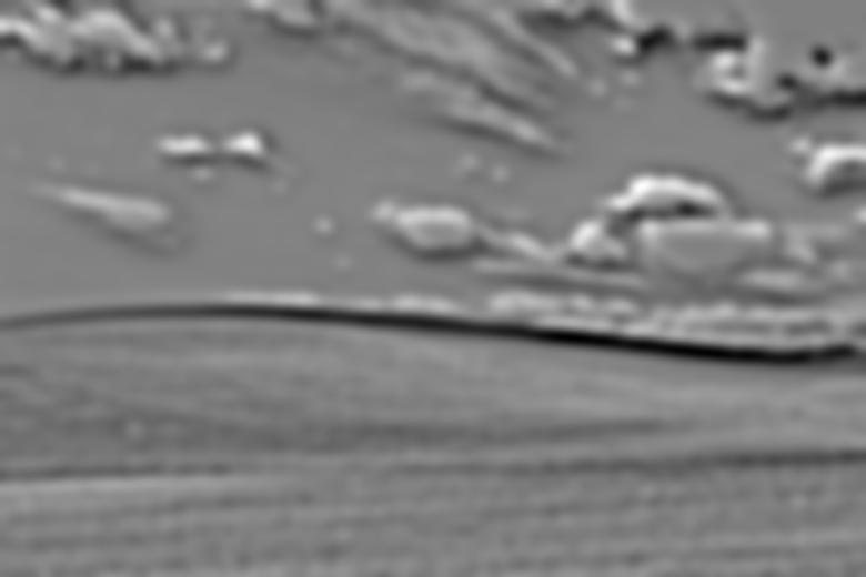
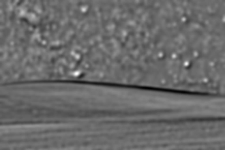
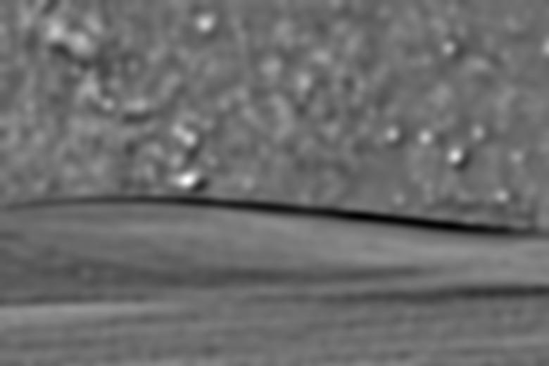
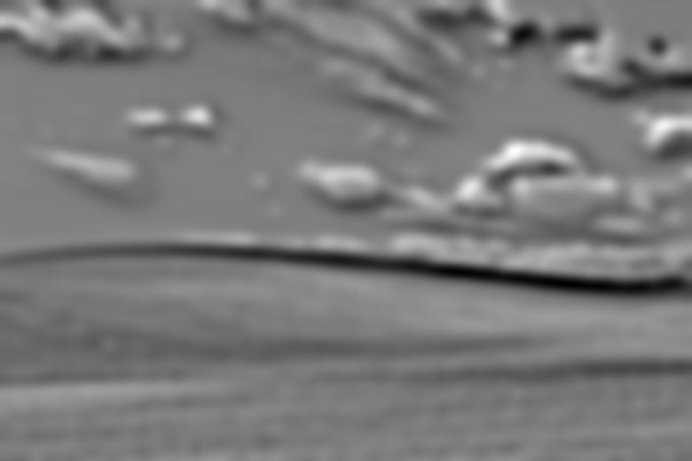
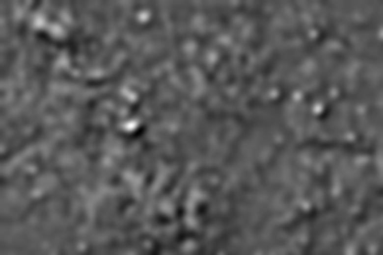
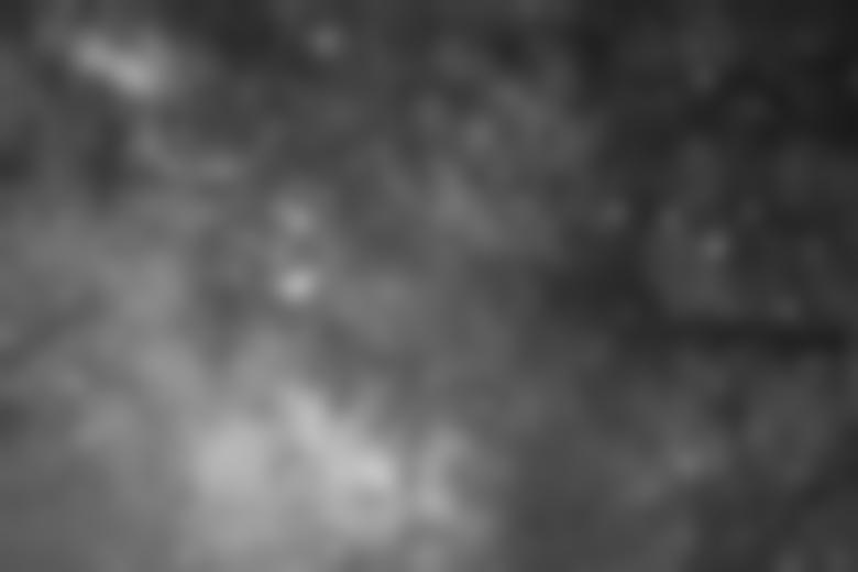
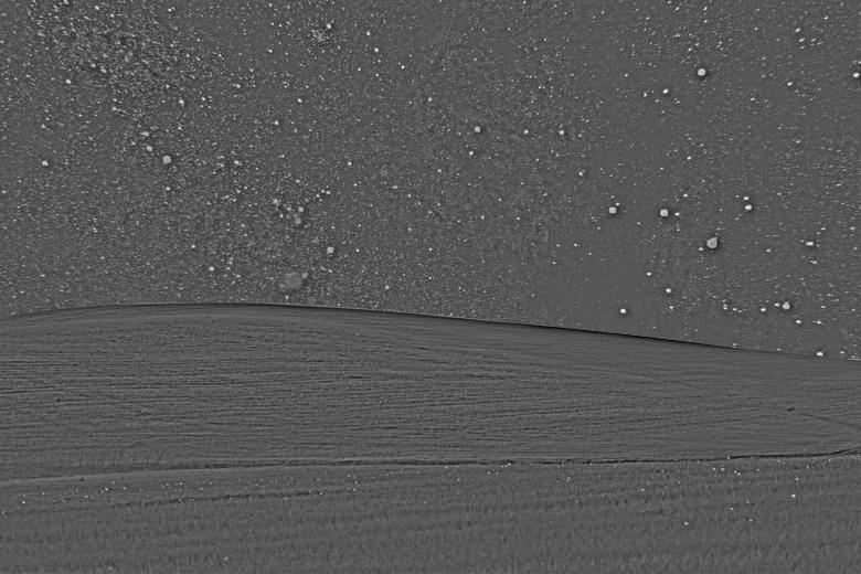
Here we have shown the guassian and laplacian stacks used to construct the blended image for the windows screensaver and galaxy images. Shown is LA, LB, GM, and LS respectively. To create the final blended image
the levels of LS were summed.
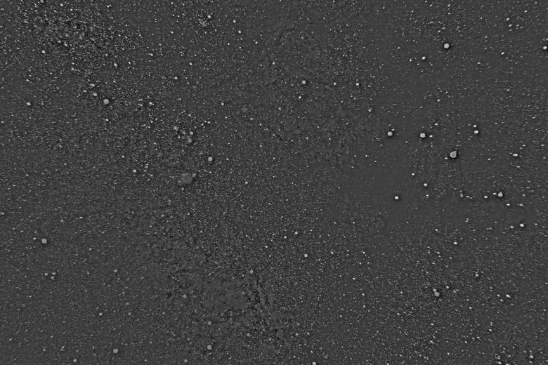
galaxy laplacian
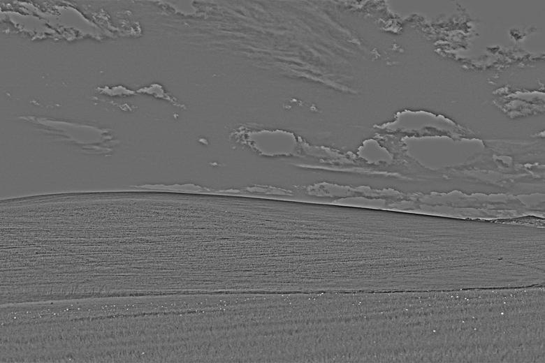
windows laplacian
mask gaussian

merged images
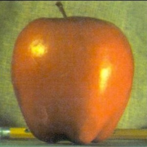
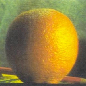
Bells and Whistles
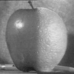
I implemented one bell/whistle for 2.4, blending the images in color. This was accomplished by blending each color channel individually and then combining them in the end. The results were largely successful.
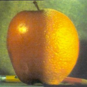
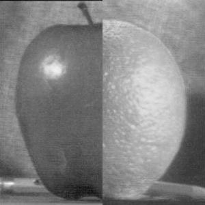
Orapple in Color
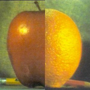
Orapple stiched together without blending in Color
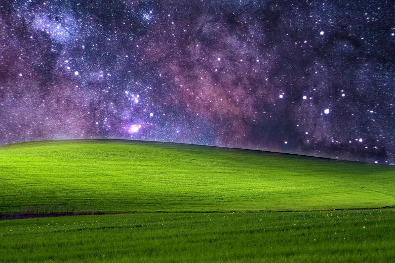
Windows Galaxy in Color
Learnings
I learned a lot from this project! I would say the most important thing I learned is exactly how powerful a Gaussian Filter is. Every single part of this project relied on the filter, and we were able to
do so many different things from the one simple concept.