Filters are linear operations that you can apply to images in order to transform the image. Filters can help provide a lot of information about the image. In particular, two special filters
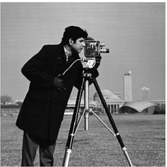
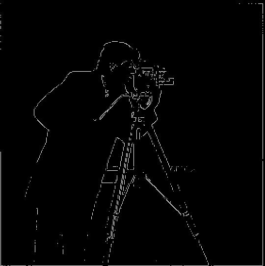
the edge detection filters can provide us with valuable information about the image, including its angles and where its edges are located. To start, consider the image below:
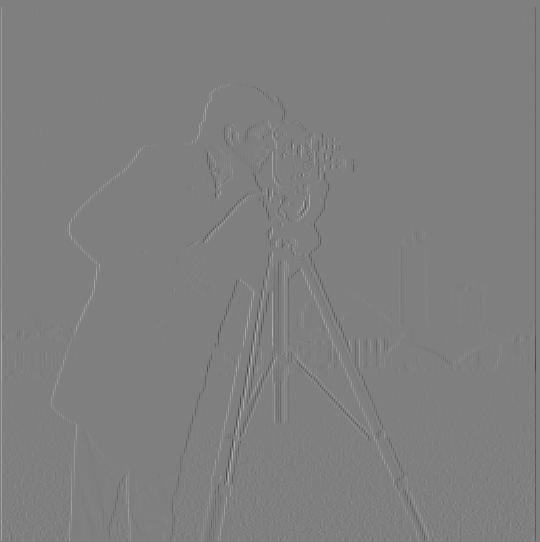
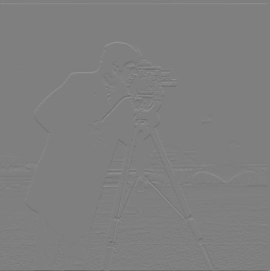
If we convolve the image, with the following two filters:
$$ D_x = [[-1, 1]] $$ and $$ D_y = [[-1], [1]] $$
we get the following outputs:
We see that as traverse our image, at edges or lines in our image, they get highlighted by black on the right and white on the left. We can use these two derivatives
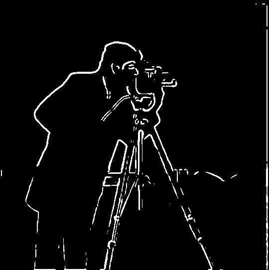
to calculate our edges in our image by simply taking the magnitude of the two images. That is,
Unfortunately, this type of filter is prone ot aliasing and high frequency noise causing random blots to appear in the image. To combat this, we can use a Gaussian Filter .
This filter is a special type of weighted filter that nicely smooths over any noise in the image. If we convolve the image with the Gaussian filter, it sort of looks like a blur. In fact,
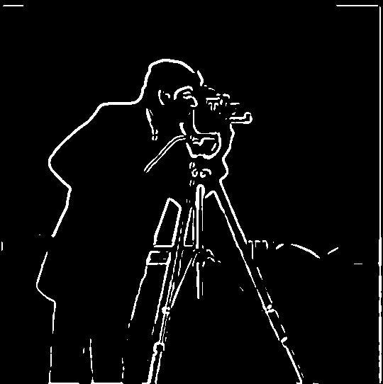
this type of blur is called a Gaussian Blur . Moreover, convolutions are commutative and associative. Thus we can either convolve our blurred image with our above filters, or convolve the gaussian filters
with the above filters before computing the gradient magnitude.
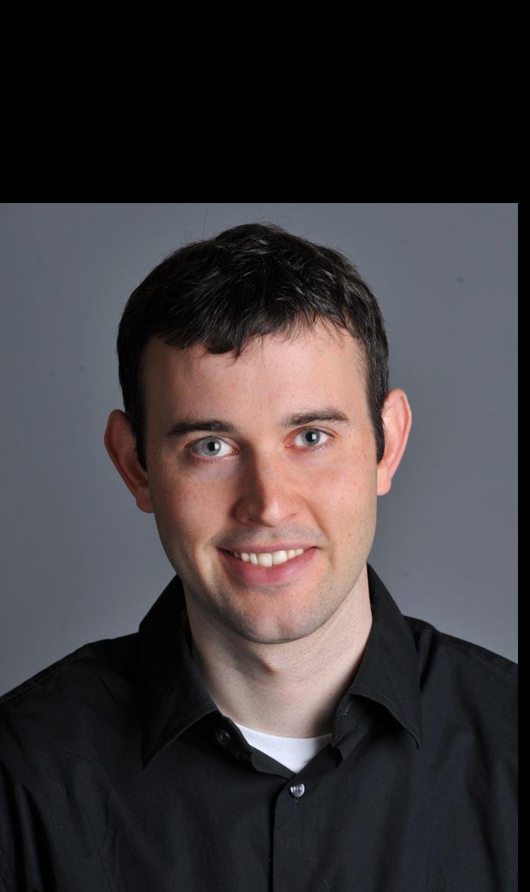
We see that this image has a lot less gunk and more defined edges than the previous blur. This helps us more concretely see where the edges are in this image which can be used
in the future for processing. Additionally, more important edges are defined. More of the man's facial features and camera features are distinguished rather than the edge features in the
background.
Image Straightening
We can also use our derivatives to apply image Straightening. Not only do we get the gradient magnitudes, but we also get the gradient angles. In general, the angle between two curves can be thought
about as the arctangent of their tangent lines slopes. Well, we just computed the derivatives (i.e slopes of the tangent lines ) for each edge. Thus, by doing the following:
$$\tan^{-1}(\frac{D_x(\text{image})}{D_y(\text{image})})$$
of our image will tell us what the angle is at each pixel. If the pixel does not correspond to an edge, we will expect garbage. But often this garbage will cancel out. We can take a histogram
of all of the angles binned at each degree to see which angles are most prevalent in the image.
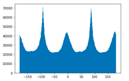
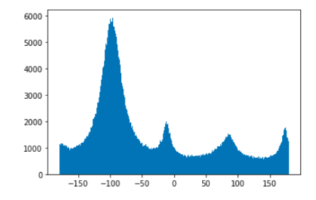
The original image is below alongside its angle histogram:
We see spikes exaclty around 0, 90, 180, -90, and -180 degrees. Which is what we expect given the image is only a "little off". In fact, we expect almost all of our images to have this type of vertical horizontal property (because of gravity). We can use this fact to
straighten our image! We can now generates our candidate rotation angles: namely
$$ \theta \in [ -10, 10] $$
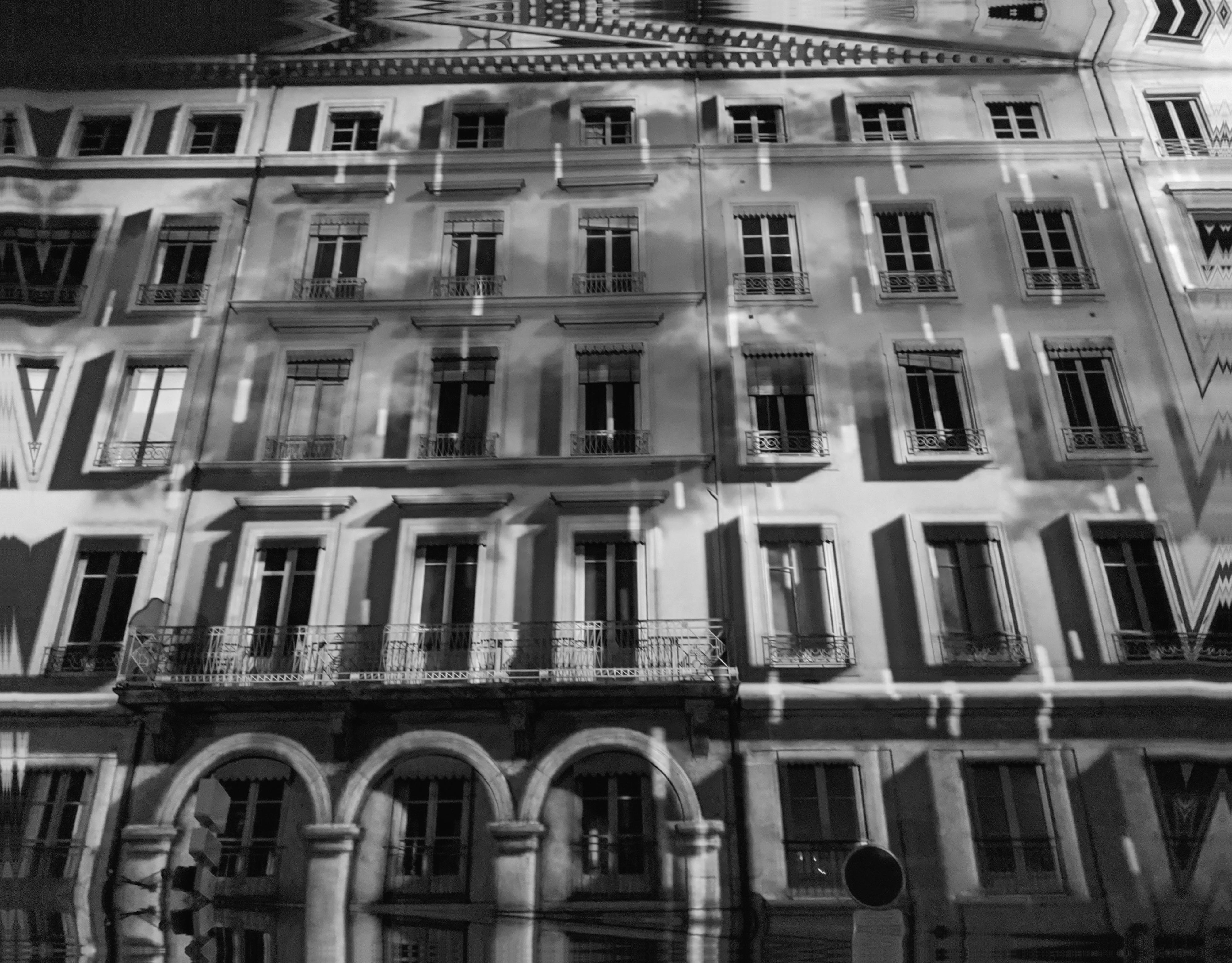
Thus, we can compute histograms for all of those angles. Then once we are done, we rank the histograms by the sum of the maxes at the 4 cardinal directions. We then take that angle and apply the rotation doing so yields:
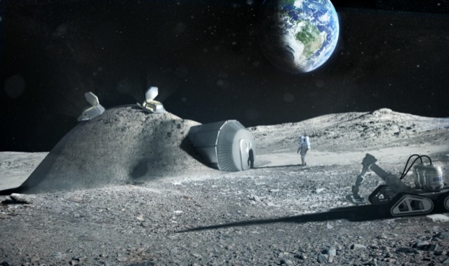
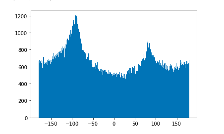
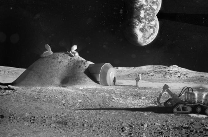
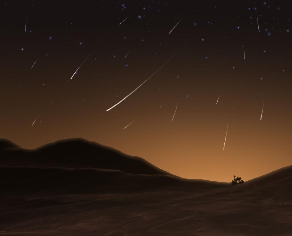
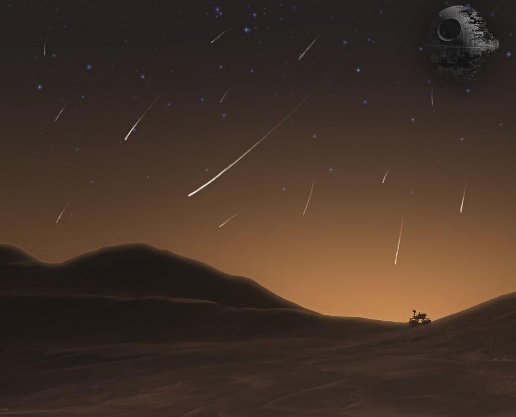
We now do this to the moon. Even on other planets, gravity is helping us determine what is horizontal and what is vertical.
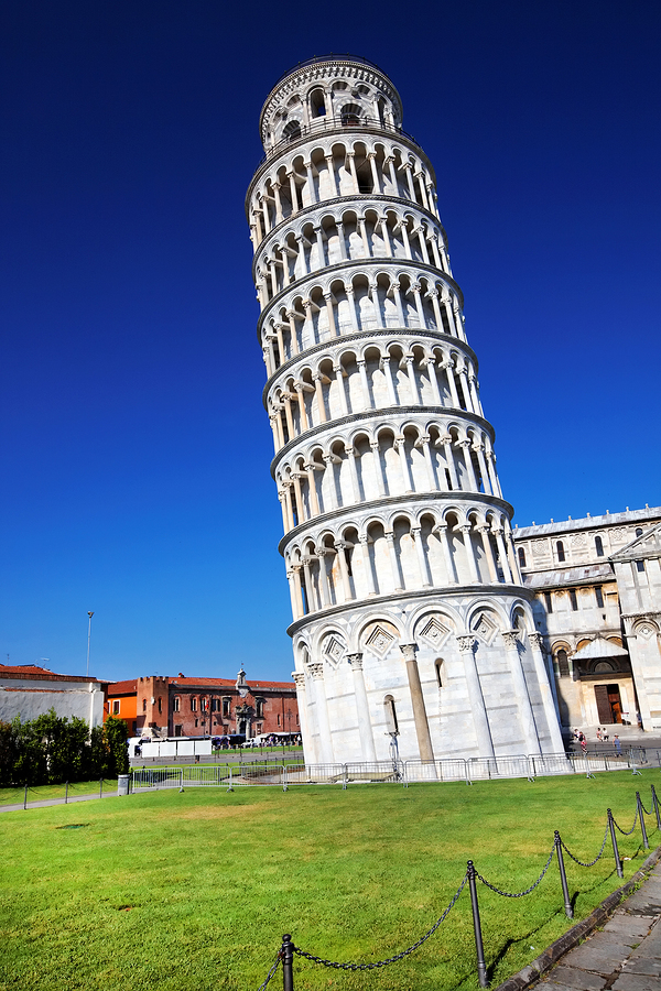
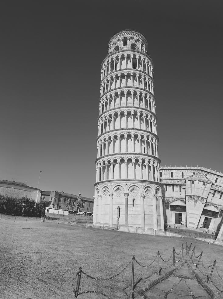
We can do the same thing for the Leaning Tower of Pisa -- or as I like to call it: the straight tower of Pisa!
In this case, we see that we have failed. Perhaps this is a pathological example of a failure, since the leaining tower of Pisa violates our assumptions that gravity tends to hold things in horizontal and vertical lines.
Hybrid Images
Image Sharpening
We have seen how we can straighten and blur and take derivatives and magnitudes of images. We now turn to how we can sharpen images. We can think about blurring images as providing a sort of
low pass filter which takes into account all of the large frequences, but not the detail of smaller ones. When we want to sharpen an image, we wnat to precisely bring out those detail in a greater fashion. Thus, if we want
higher frequencies, we should take the original image, and subtract out our lower frequencies to get higher ones.
In particular, we will use the following formula
$$ I_{\text{sharp}} = (1 + \alpha) \cdot I_{\orig} - \alpha \cdot I_{\text{blur}} $$.
Since convolution is linear this is the same as
$$ I_{\orig} * ((1 + \alpha) Id - \alpha \cdot \text{Gauss}) $$
where Id is the identity convolution and Gauss is the gaussian convolution filter.
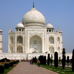
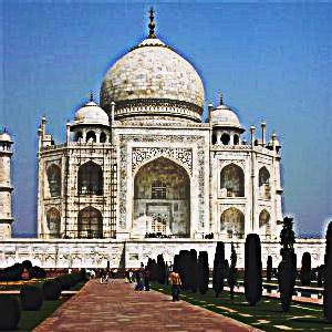
Doing so on the Taj Majal image below, one can see a striking difference:
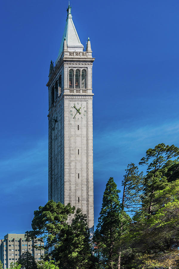
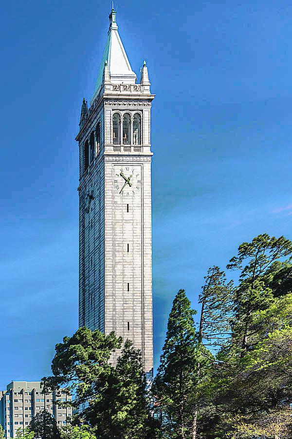
We do this again, except this time with a more Berkeley themed object:
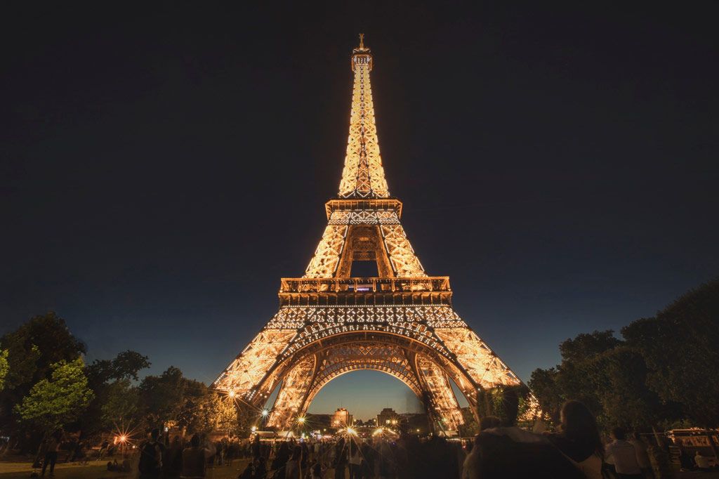
What happens if we blur and image and then try to sharpen it? Well, consider the image below of the eiffel tower:
If we are to blur and then re-sharpen, we actually won't see a big difference. This is because we have already thrown away the higher frequency information when we did our convolution. This means
we can't get that information back, and so any sharpening will only keep emphasize highest frequencies of the blurred image, rather than the highest frequencies of the origina limage. Nevertheless, this yields
an interesting effect. (Blur on left, blur-sharp on right).
Hybrid Images
Now that we have worked on image sharpening, we can try to take aim at doing hybrid images. Remember, we saw that we could make a distinction between low frequencies and high frequencies in the last image. What happens
when combine two separate images with different frequences. The result is that close up you see one image, and far away you see the other. To illustrate this, look at the example below:
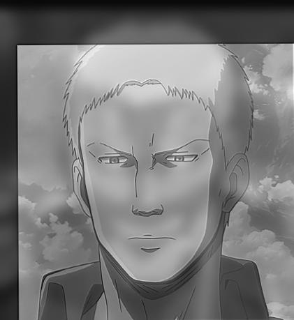
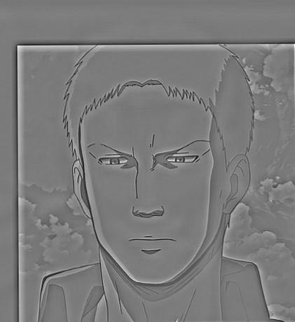
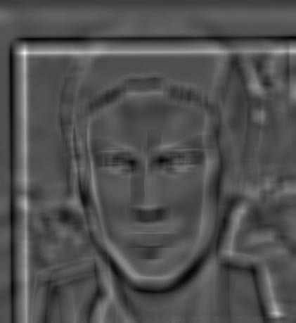
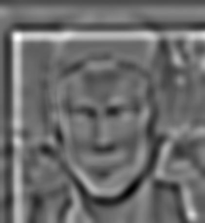
Another example comes from the popular anime Attack on Titan. We create an image blending between Reiner and his titan, the Armored Titan.
Other Hybrid Images
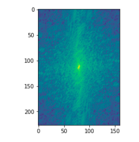
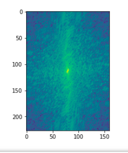
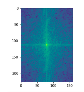
This case is interesting since it demonstrates very clearly how the frequency domain plays a role. Let us look at the fourier transforms at each stage of this hybridization.
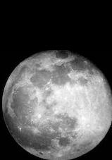
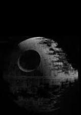
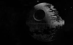
First, we calculate the fourier transform of the original two images, the moon and death-star respectively:
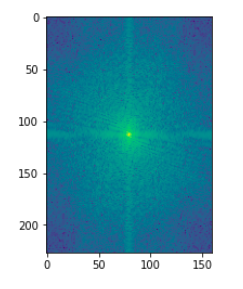
Now, we look at the Fourier transform of the low pass blur of the moon and the high pass sharpening of the death star.
We see that the fourier blur has almost no high frequencies and almost all frequencies are concentrated around the origin or the axis. In contrast, the frequencies of the
sharp image are distributed relatively evenly across the entire domain. We still expect a lot of small frequencies near the origin, but this is different since the frequencies are more evenly distributed than
normal.
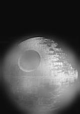
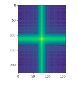
Finally, when we blur the image something happens:
Now we see both high frequency distributions and low frequency distributions. THis corresponds to the higher and lower frequency parts of the image and is why the image looks like the death star from up close
and the moon from far away.
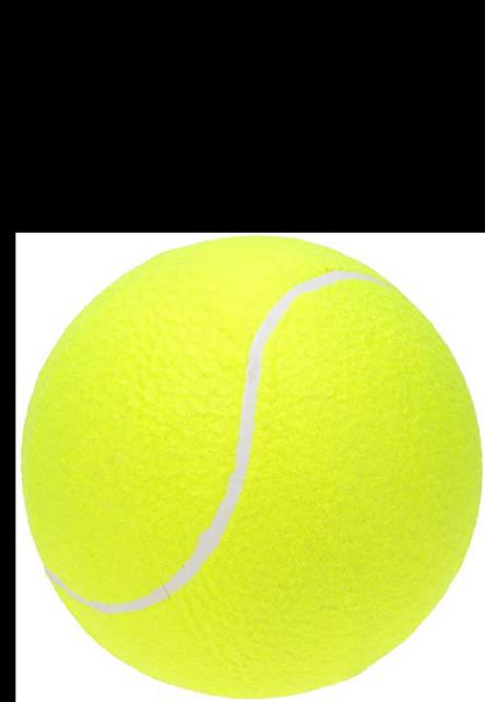
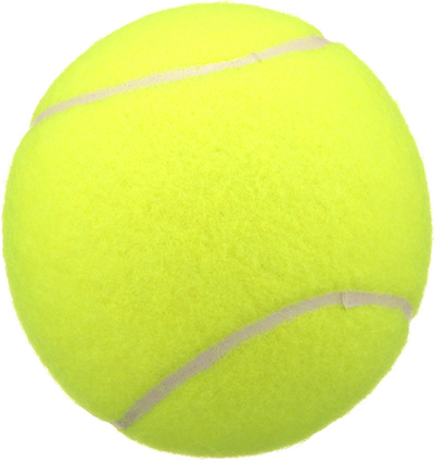
This one below is a failure case. The images are simply too similar and don't have that much variation in frequency, so it is very easy to tell them apart from afar. The
tennis ball, in particular, has very little that can be done via sharpening.
Gaussian and Laplacian Stacks
What happens when we keep applying filters to an image and keep convolving it down. Then, we end up with a Gaussian Stack. If we keep applying filters from the starting image
moving down, each image in this process is an image in the stack. These images represent smaller and smaller frequencies as they get convolved down. If we subtract the images
from each other, we get what is called a Laplacian stack. These images represent the set of images in a band of certain frequencies.
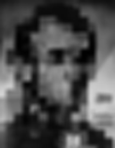
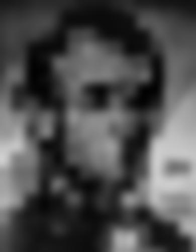
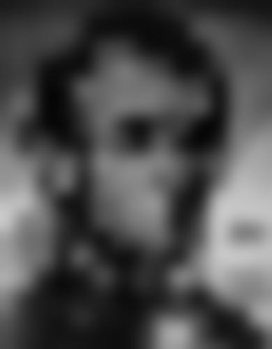
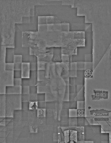
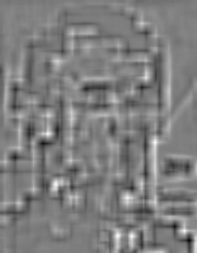
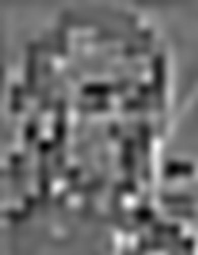
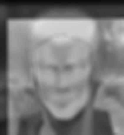
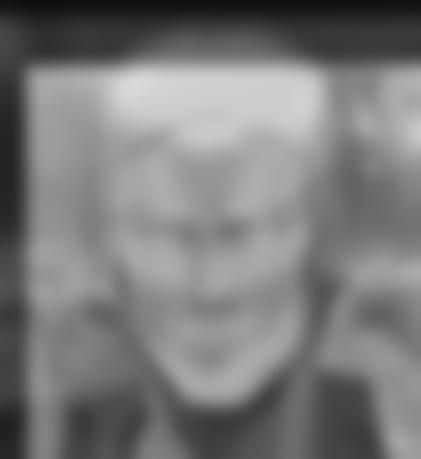
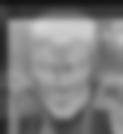
As an example, let us consider the lincoln picture below.
Now, let us apply the Gaussian and Laplacian Stacks:
In the highest frequencies of the laplacian we are able to see the lady, whereas as we go lower and lower into the frequencies, the image starts to look more
and more like Lincoln.
We do the same thing with our previous image pyramid using Reiner and the Armored Titan to explain what is happening with those images:
Now, let us apply the Gaussian and Laplacian Stacks:
This clearly shows us what is happening at the frequency level for hybrid images. At the higest frequencies we have Reiner and at lower ones we have the Armored Titan.
This explains why at a lower resolution or from far away, the picture looksl like the titan versus looking like Reiner.
Blended Images
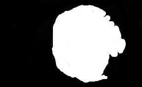
We can now use our techniques built up so far to blend images togther in really interesting ways. Given a two images and their laplacian stack, we can compute a mask of
an image we want to blend in with another image. Then, we make a gaussian pyramid of the mask. If we have a stack size of $N$ and and two images $I_1$ and $I_2$ and mask $M$, we can
compute the blended image as follows:
$$ I_{blend} = \sum_{i = 1}^n Lap(I_1, i) \cdot Gauss(M, i) + Lap(I_2, i) \cdot ( 1 - Gauss(M, i)) $$
Where $Lap(I, i)$ is the $i$th image in the laplacian pyramid and likewise for the gauss. Here are the results:
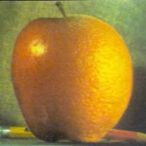
The Orapple
In this case, our mask was simply a half white, half black image.
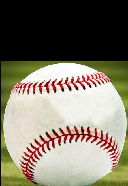
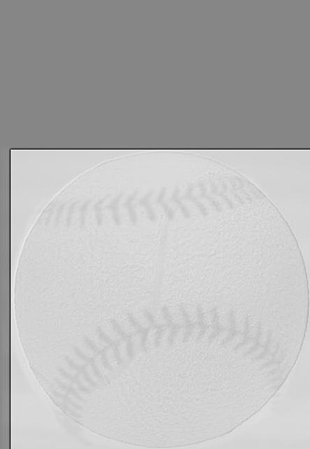
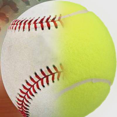
Baseball - Tennis Revisited
Let us try our luck at this combination again. This time we will see a blended image between a baseball and tennis ball. Once again, here our mask was
simply a half-white, half black image.