In this part, I have explored the magic of using a basic filter and convolution technology to get some properties of the image such as derivatives and further calculate the gradients. Combined with it, I have also explored the gaussian filter in some ways.
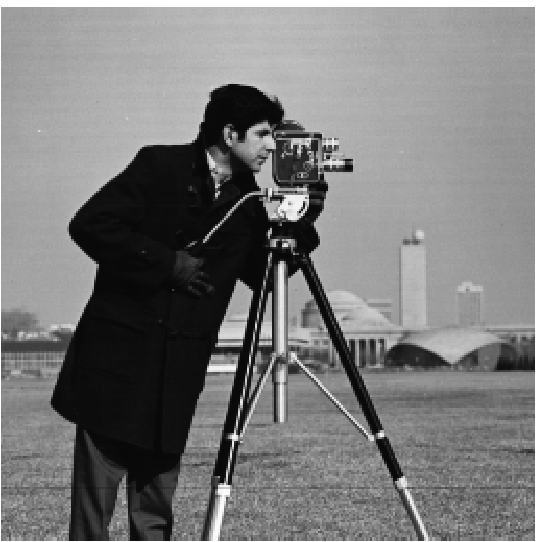
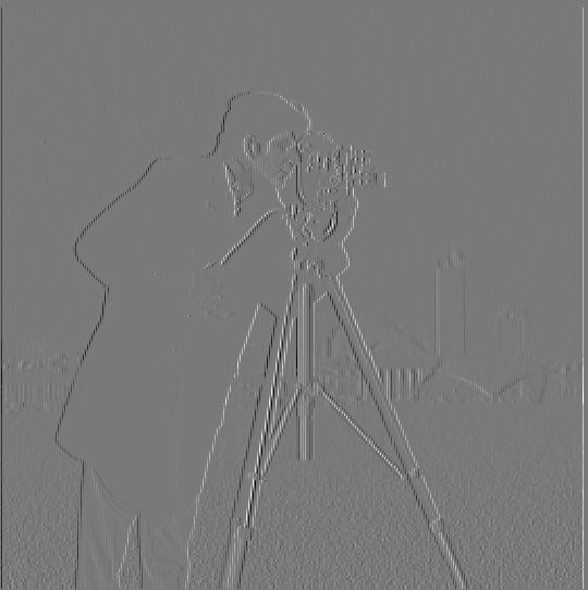
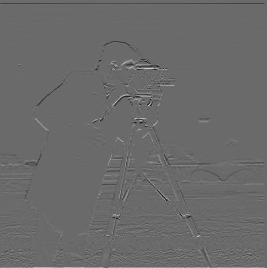
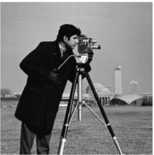
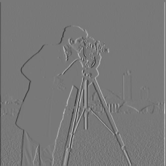
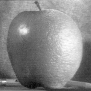
The first part is to play with the basic filter of derivatives in both x and y direction on an original cameraman image.
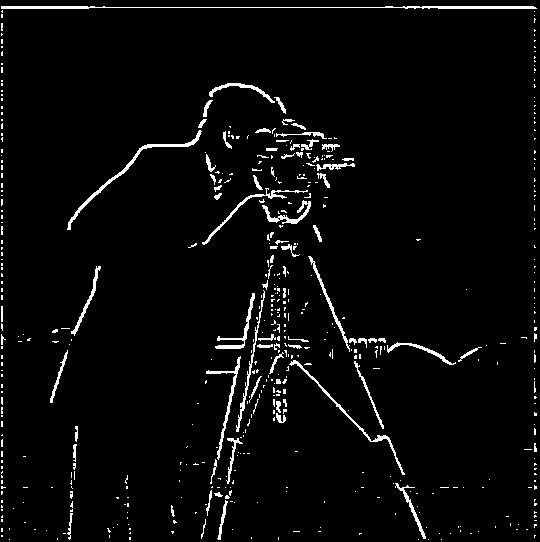
First, I used dx = [1, -1] and dy = [1, -1].T to convolute with the original cameraman photo to get the derivative of x and y. Second, I computed the magnitude of the gradient using the formula np.sqrt(dx^2 + dy^2). Third, I computed the magnitude of the orientaion of the gradient using the formula np.arctan2(-dy, dx). (The grdient is imploved by setting values greater than a certain threshold to 1 and 0 for values under the threshold.)
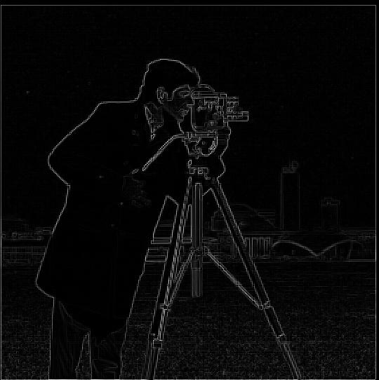
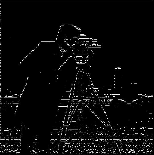
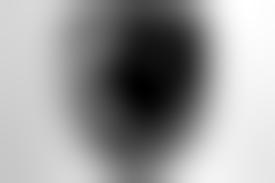
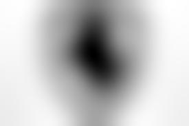
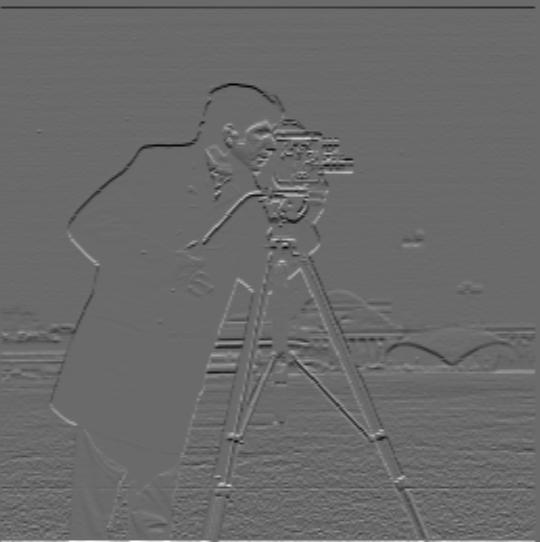
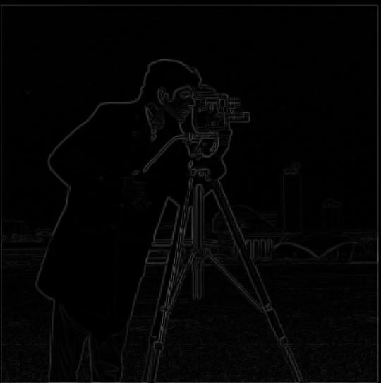
For this second part, I have explored the power of Gaussian filter by first using it to blur the image and then calculate the derivatives.
First, I convoluted the original cameraman image with a Gaussian filter of size of 5 and sigma of 1 to blur it. Then, I applied dx and dy filter and calculate the derivatives as previous part. After that, with the properties of convolution, I change the order of calcultion by first convolute the Gaussian with the derivative filters and then applied the whole filters to the original image. And being verified, we get the same results (with some variation since I used a threshold).
What we can see about the advantages of using gaussian filter is that it filters out the very high frequency features of the image such as the grass in this photo (for the one didn't use DoG, the grass part has all those small dots). Because of that, the gradient will show clearer and more obvious edges like we human can see.
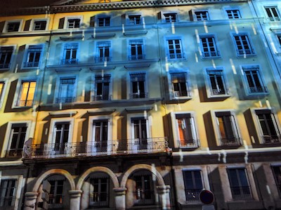
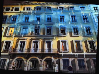
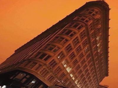
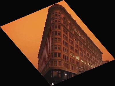
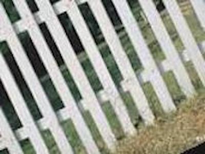
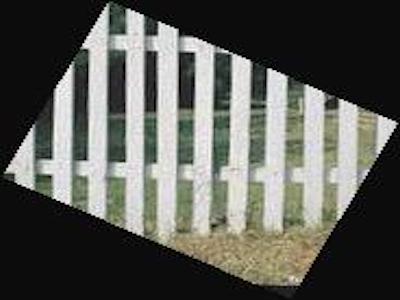
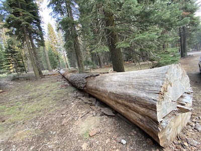
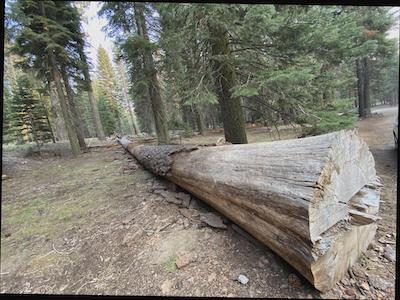
This part is pretty fun. It enables us to "straighten" a image. By "straighten", it means to get the horizontal and vertical lines maximized. Then, how should we detect those horizontal and vertical lines and see if they are straight enough?
The idea if to use the previous parts filters to calculate the gradient and orientation of the image and using a range search of angle to determine the angle with the most percentage of "valid" edges in a selected region.
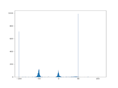
The specifc process I used is: First, apply the image with the DoG and calculate the gradient including its magnitude and orientation. Second, I transfer the orientation in range [-pi, pi] and used a helper function to count all the edges that lies in the range I set [-185, -175], [-95, -85], [-5, 5], [85, 95], and [175, 185]. Third, I used a loop in a certain range of angles to search for the best one by calculating all the valid edges in a selected region. The region needs to be selected at the part that potentially has more horizontal and vertical lines. The region also needs to be at middle of the image to avoid edge effect of rotating of an image. I didn't search for a whole large range of angle but instead using a range of around 30 degrees. We can select the range by first visually determine the approximate angle or doing more sets of calculations by moving the range around.
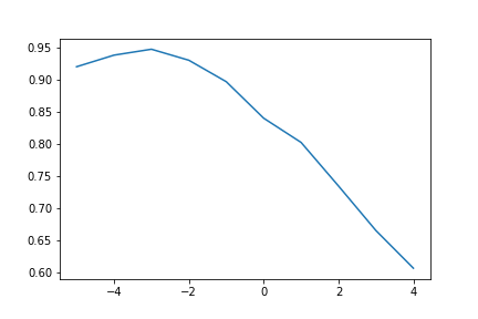
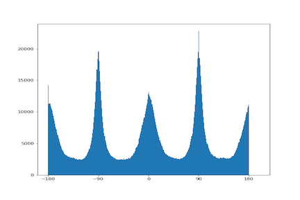
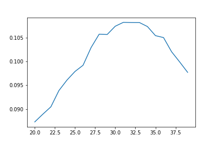
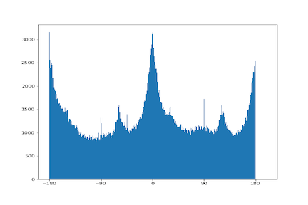
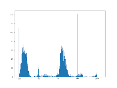
We can see for the degree with the highest percentage of valid edges, there are modes for the edge histogram at [-180, -90, 0, 90, 180], which is very reasonable at we predicted.
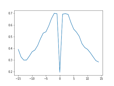
The following image of a trees is a failed case. Looking through the edge plot, one reason may because there are lots of branches, which is pointing to different orientation and the method we are using just choose one direction of which the most of the branches pointing at, which is not the case we want.
One possible solution for this,I believe, is to use a gaussian filter with higher sigma to filter out more branches. However, that may cause too many being filtered and left only very few features for us to calculate on.
For this part, we need to "sharpen" the image by bringing more wight to its edges. We can do this by using the Gaussian filter, which has the property to filter out the high frequency of the image. Therefore, by substracting that from the original image, we can get the part being filtered out, which is the high frequency part that we want. After that, just add that high-freq part to the original image, we will get one new image with edges being sharpened.

For this part, we used the idea from SIGGRAPH 2006 paper by Oliva, Torralba, and Schyns to hybrid two images into one in a way that when people look at a closer distance, they will see one image while look at a far distance, they will see the other image. The magic behind that is to play with the frequencies so that one image occupies the high frequency range while the other possesses the low frequeny. When people look from a closer distance, the eyes distinct the high frequency more while from a large distance, the eyes can only tell the difference that happens in low frequency.
Hence, we only need to find a way to extract the high frequency and low frequency and join them together under a certain weights. We can do that using Gaussian filter because again, it's the magic tool to filter out the high frequency and substract that we can also get the high-freq part as well.
The specifc process I did is: First, picking two points from each image that I want to combine so that later I can use two points to align and anchor the images. Second, I used the python starting code to align the image. Third, I applied the Gaussian filter to get the corresponding low and high frequency of the images. Last, I joined the low and high "parts" of the images together using a certain weight.
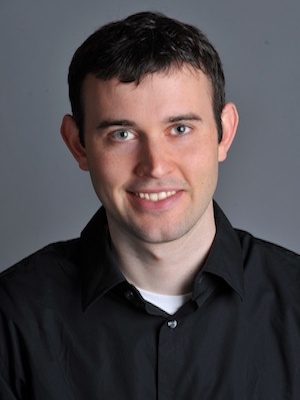
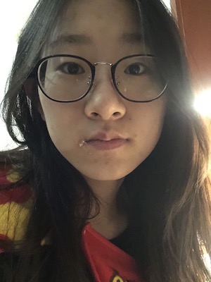
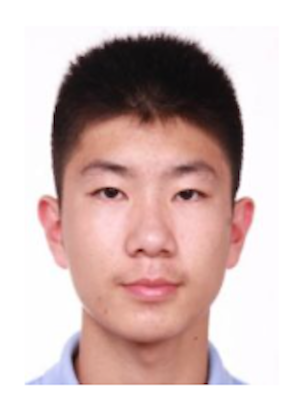
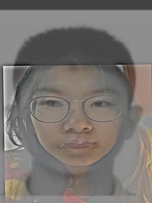
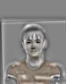
Below is the hybrid of the image of my sister and an image of myself. Finally realize how close we look like.
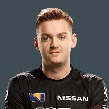
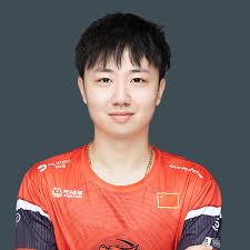
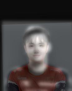
The hybrid of my favorite CS:GO players Niko and Somebody. Got to admit, somebody really has some "high-frequency" features.
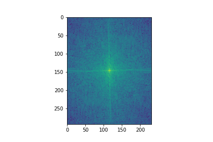
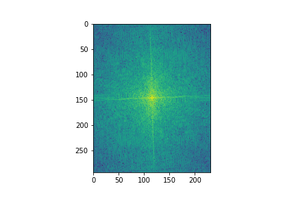
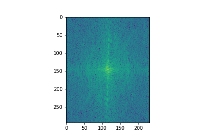
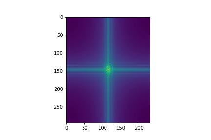
Let's see the log magnitudes of their Fourier transforms.

I tried to apply the color for the high freq part as showed two images above. I think it looks better because it amplifies the high freq part when we look at closer distance. when we look from a very far distance, we still can't see those high-frequenct edges.
In this part, I explored the Gaussian and Laplacian Stacks. The stacks are just like a pyramid but without downsizing. The sigma of the Gaussian filter is the one that increases with the layer.
For the Gaussian stack, it's just a stack of images that uses different value of sigmas, which are increasing with the layer.
For the Laplacian stack, it composes of images from the difference of each consecutive layer image of Gaussian stack. The stack has the property to investigate on features at different frequencies.
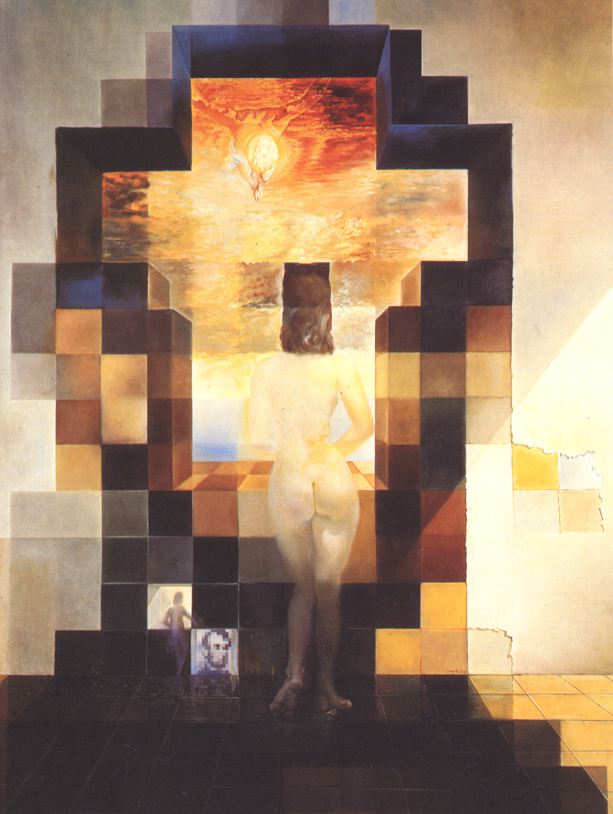
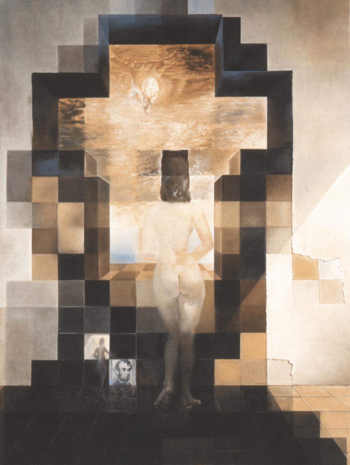
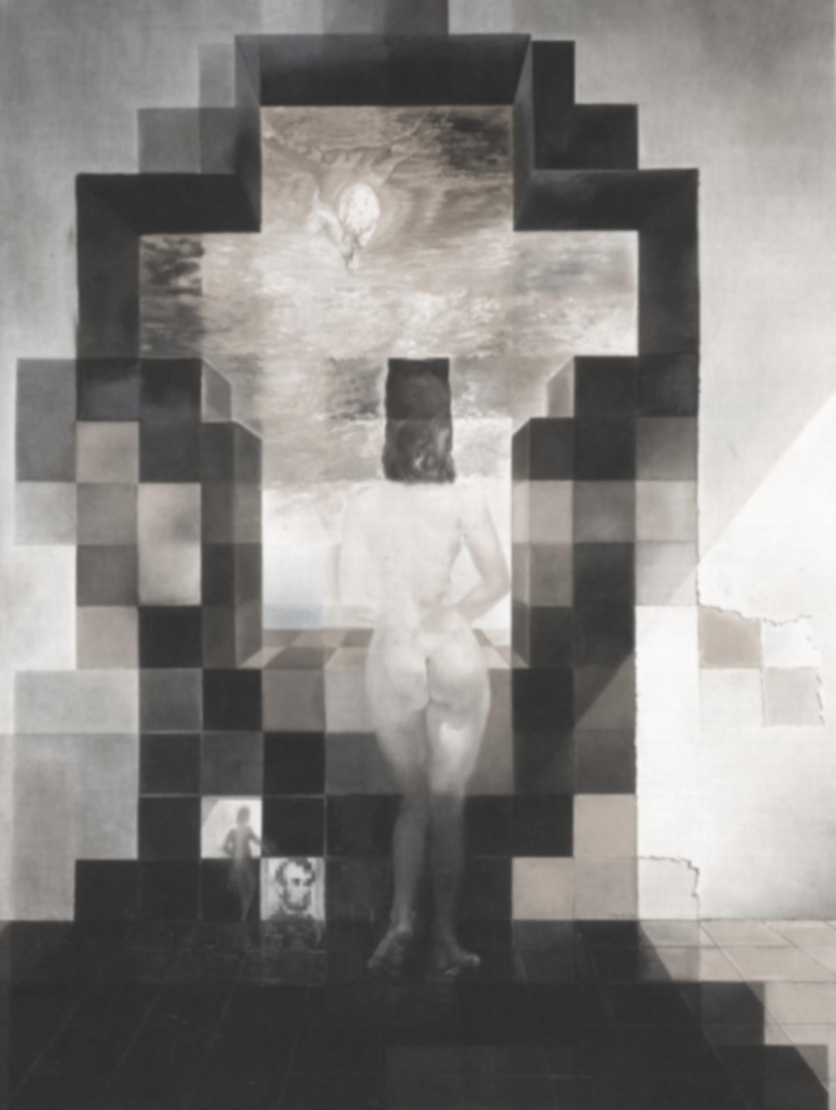
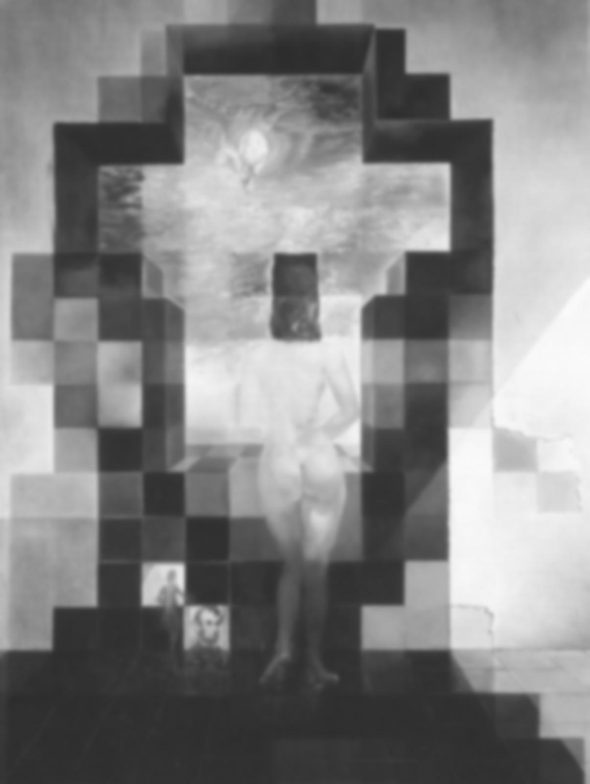
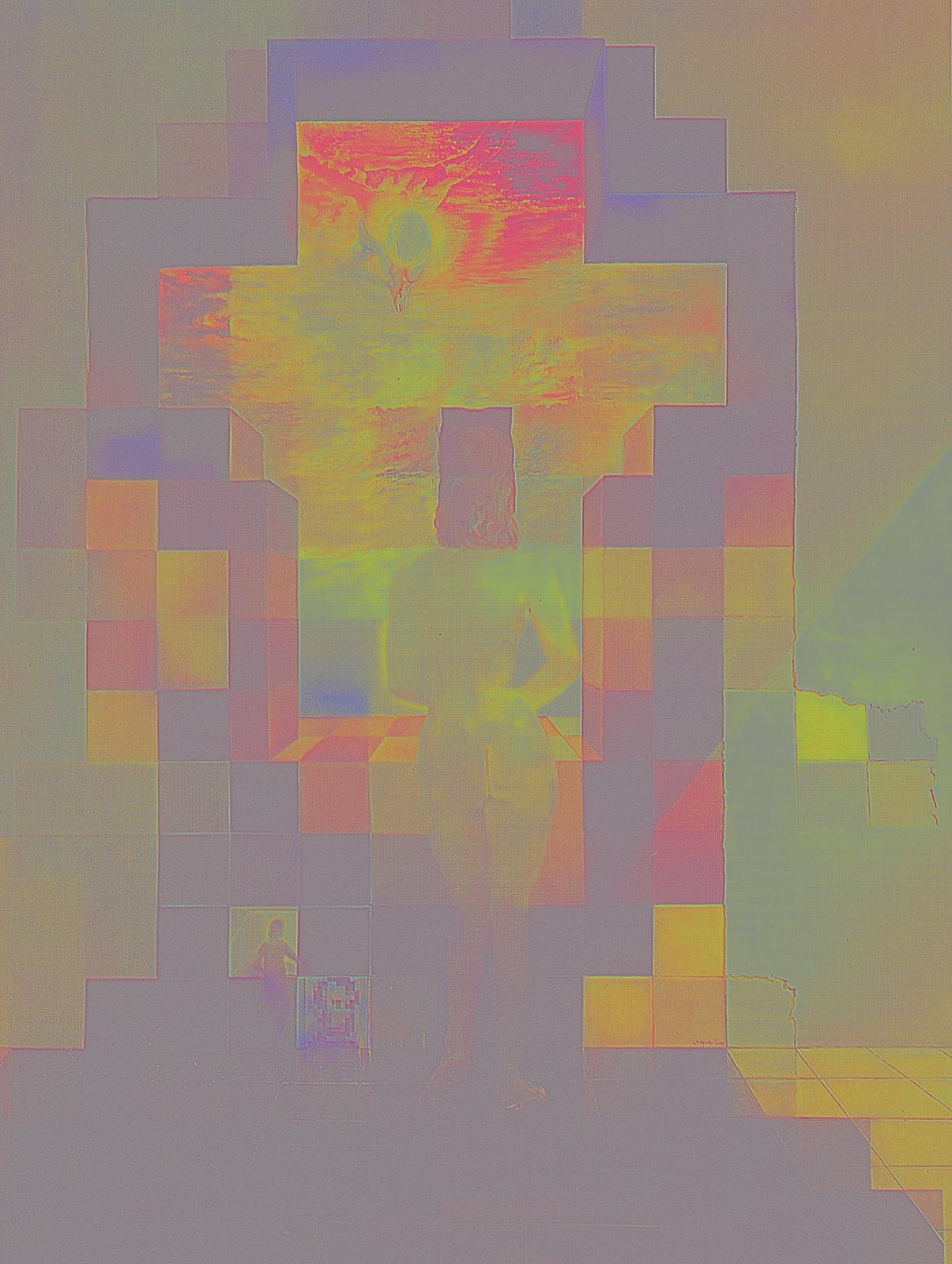
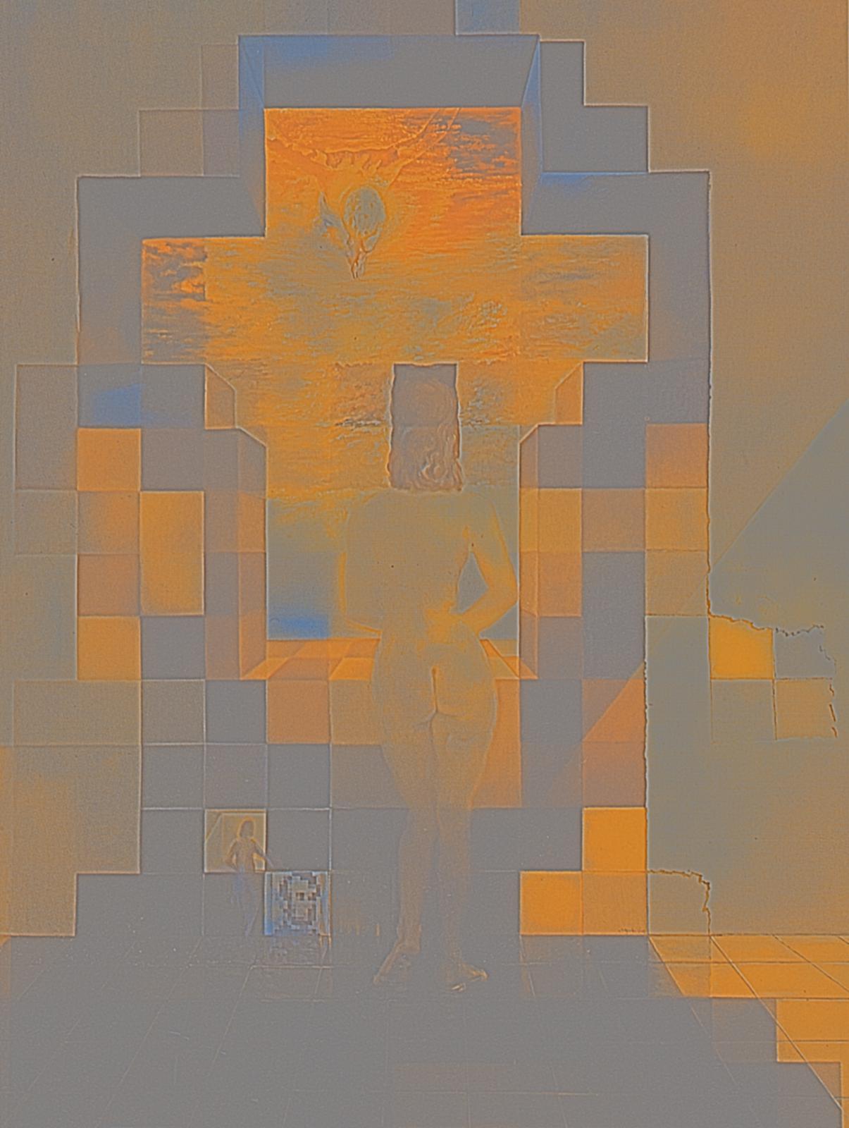
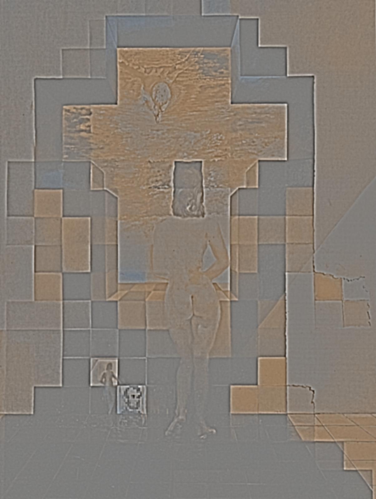
The followings are the Gaussian and Laplacian stacks of the Salvador Dali's painting of Lincoln and Gala using original sigam of 1 and factor of 2 over layers.


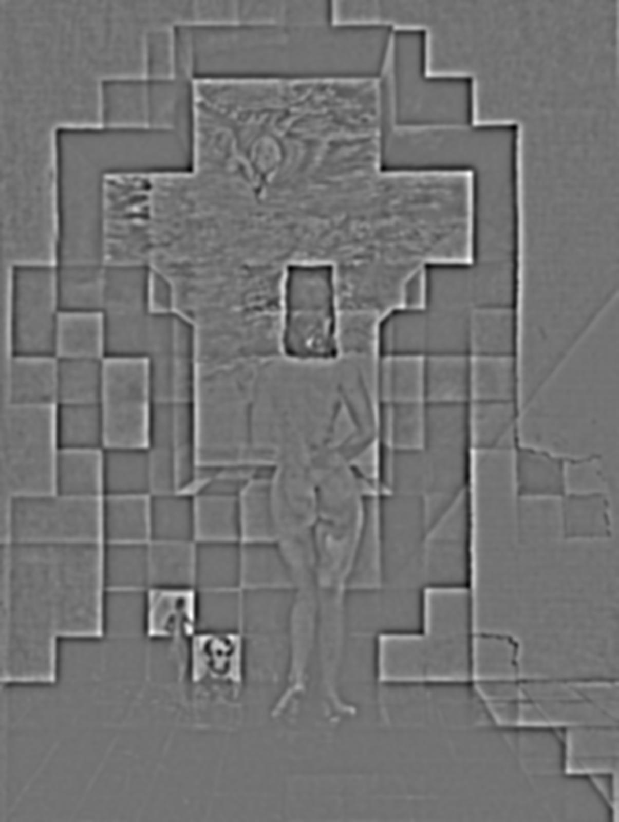
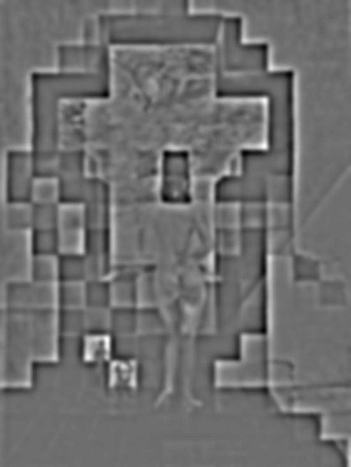
The followings are the Gaussian and Laplacian stacks for the hybrid image "SomeNiko"
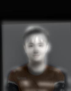
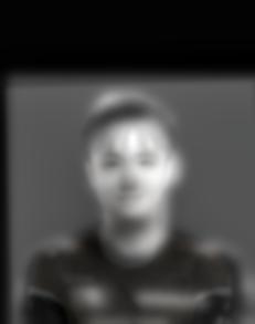

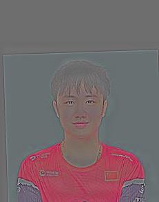
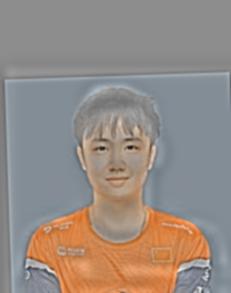
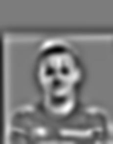
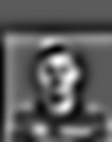
We can see that niko's image is very blurred just at the third level of gaussian while somebody's features are still clear to see in deeper level for example the hair.
I think this is because the gaussian sigma is too large for niko's image so its features are quickly being filtered. One way to solve this, I think, is to adjust the sigma values for niko's image.
In this part, we try to blend two images together. Different from the hybrid idea, we want the seam between two images be as natural as possible.
The idea to achieve that is to use different indecies for different freqencies of the images so that the higher freqency has more sharp in indecies around seam region while for lower frequencies, we let them knid of stretch out a little bit to blend within each other. Since they are low freqencies, the eyes won't tell much difference at the overlayed part but that will still smooth the seam.
To make it practical, we need to choose a mask first and used Gaussian filter to calculate the Gaussian stack of it, which will then be used as the weight of multiplication for each layer. Then, we just need to calculate the laplacian stacks for each image and muptiplied each with the corresponding mask. Then, we can directly add each image at each level to get the laplacian stacks for the blended image. Last, we can just stack all the layers in the laplacian stacks together to get the final blended image.


Below is the blended image of the logos from my hometown basketball and football teams: Beijing Jinyu and Beijing Guoan