CS 194-26 Project 2: Fun with Filters and Frequencies!
2020 September 22, cs194-26 (Kecheng Chen)
Part 1: Fun with Filters
In this part, I will deal with 2D convolutions and filtering.
1.1: Finite Difference Operator
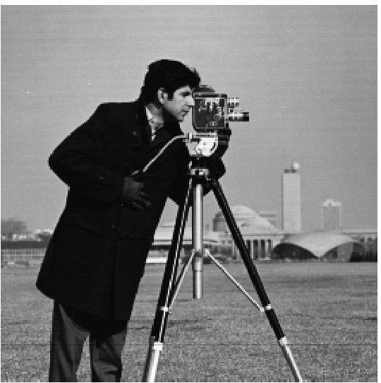
Consider an image as a 2D function f(x,y), we could approximate the partial derivative using finite differences. Filters here are D_x=[1 -1] and D_y=[1 -1]^T. Then I used each filter to do the 2D convolution(conv2). Image size is 540*542. Results are shown below.
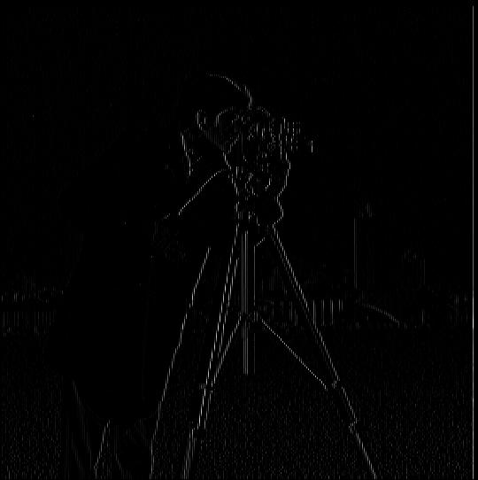
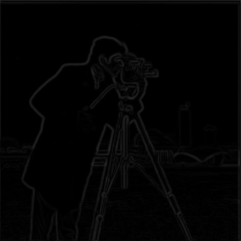
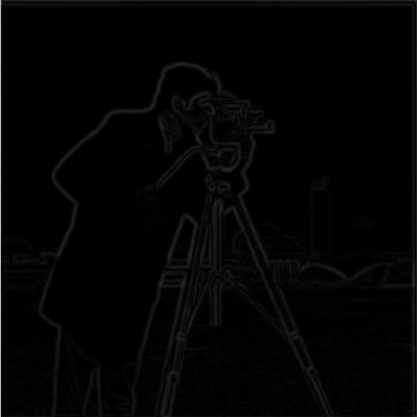
Then I calculated gradient magnitude using sqrt(D_x^2+D_y^2). In order to get edge image, threshold needs to be set to binarize gradient magnitude image. I used 0.2 as threshold, which would somewhat suppress the noise and not lose edges interested.
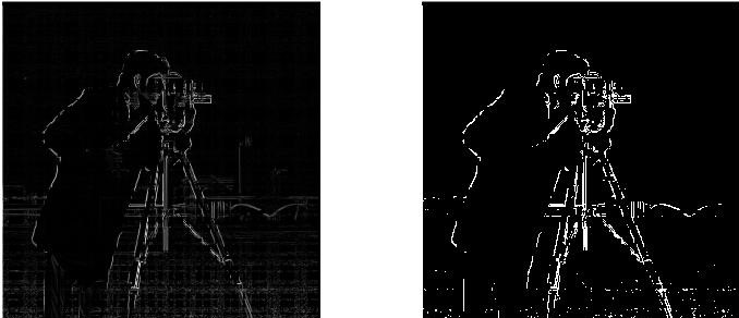 Gradient magnitude and edge
|
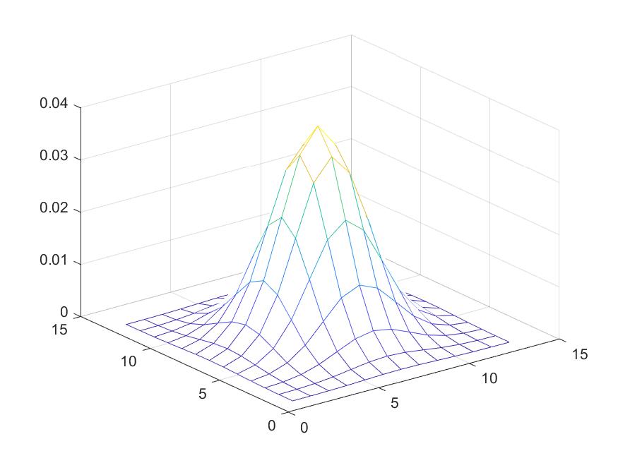
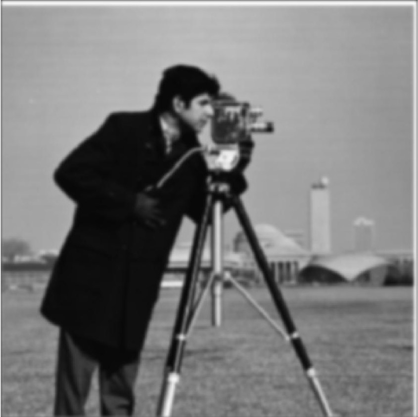
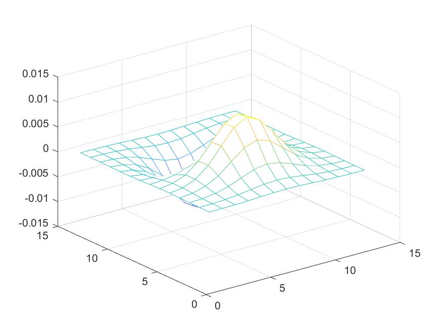
1.2: Derivative of Gaussian (DoG) Filter
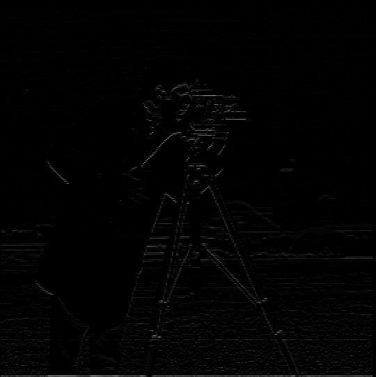
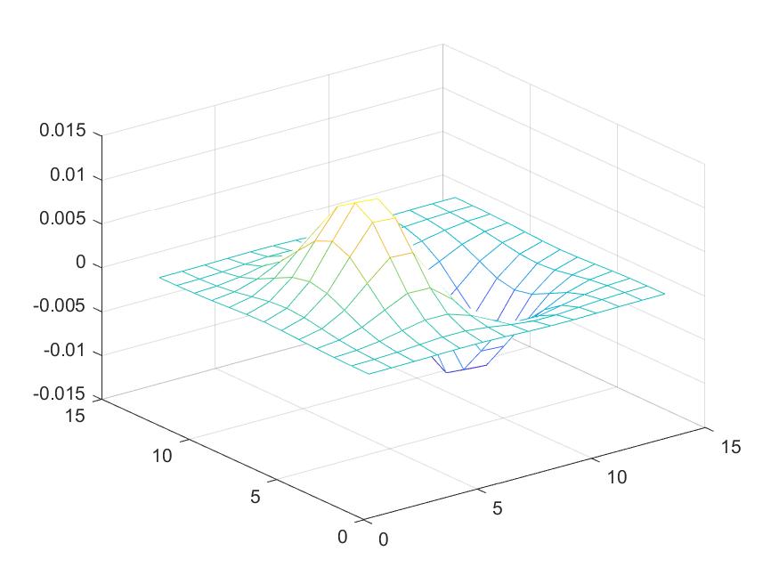
The above result is somewhat noisy, so here we need smoothing operator: the Gaussian filter. Then i defined a Gaussian kernel with sigma=2 and half-size=2*3=6. A blurred version of the original image is created after the convolution. There is a significant difference. For the present result, edge is much smooth and noise is largely suppressed compared with the previous one. The effect of manually setting threshold is bad. There is a trade-off between maintaining edges and suppressing noise. Then follow the same process as the above. The result is much better.
 Gaussian kernel
|
 Blurred image
|
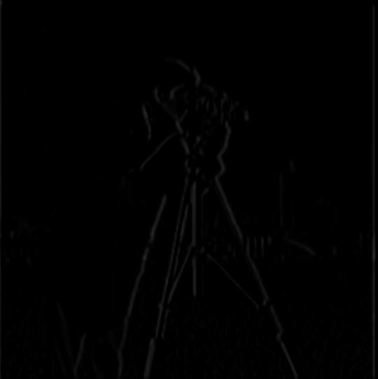 D_x
D_x
|
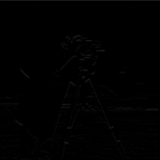 D_y
D_y
|
 Gradient magnitude
|
Based on the commutative and associative rule of the convolution, I can convolve the gaussian with D_x and D_y first and then applied them to the original image. The result is the same as before.
 D_x*Gaussian
|
 D_y*Gaussian
|
 Gradient magnitude
|
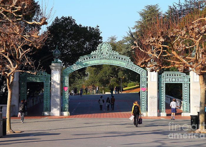
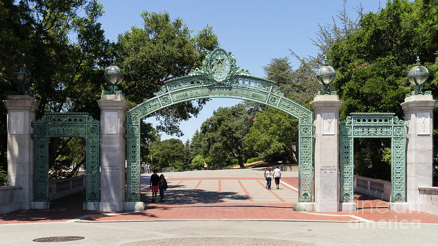
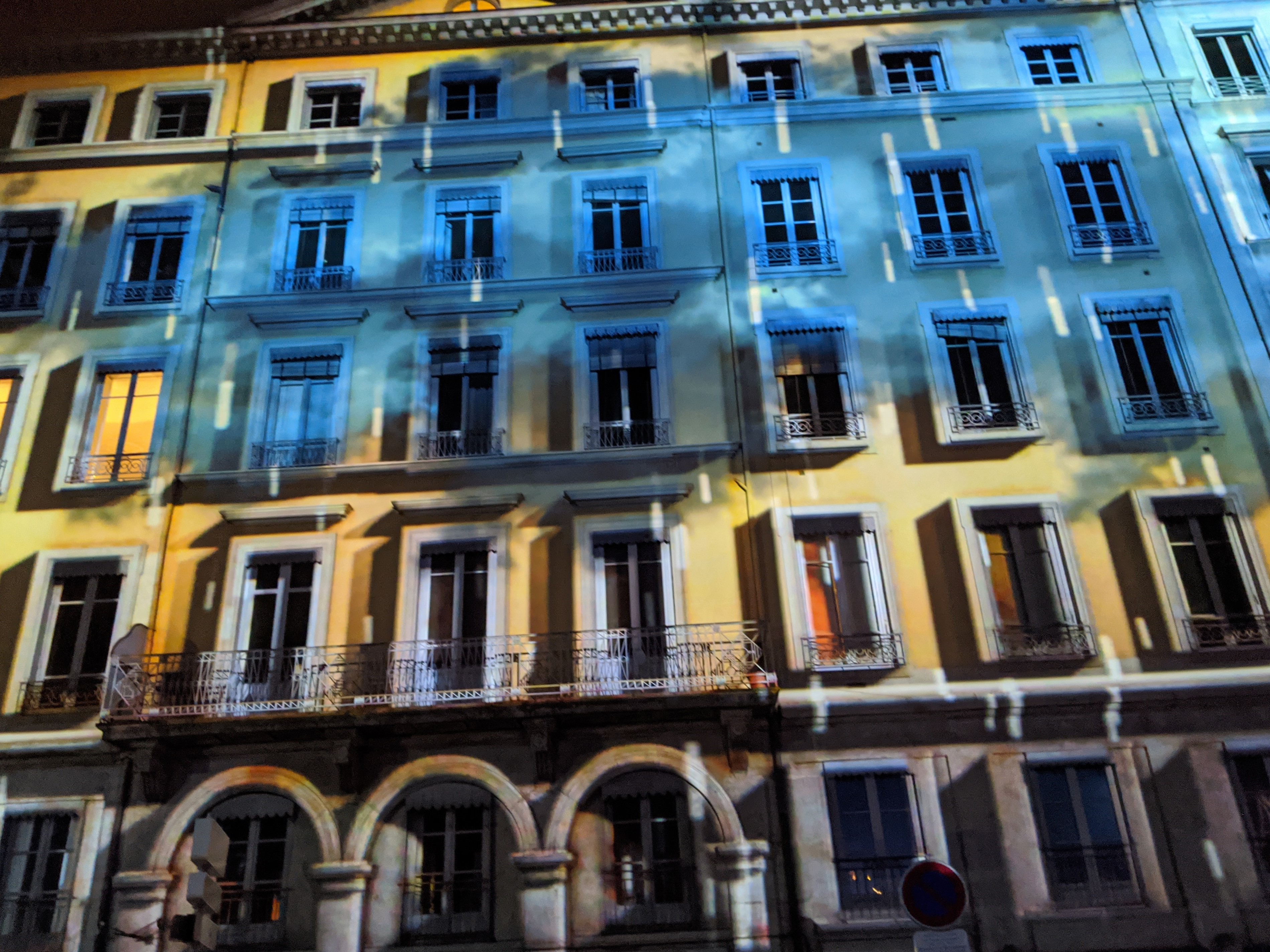
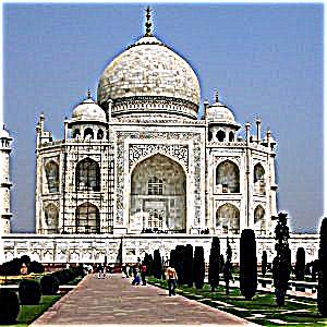
1.3: Image Straightening
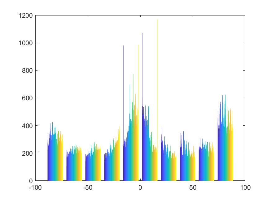
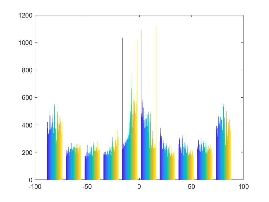
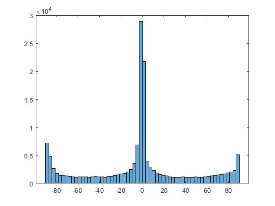
There are artifical edges created when rotating the image, so i cropped image with 20 percent after each rotation of the original image. Then i draw the histogram of each image and found the best rotation with the maximum number of angles located in the predefined range [-5 5], [-95 -85] and [85 95].(horizontal and vertical edges)
 Original image
|
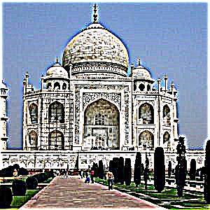
 Result image
|
 Original_crop
|
 Original_histogram
|
 Result_crop
|
 Result_histogram
|
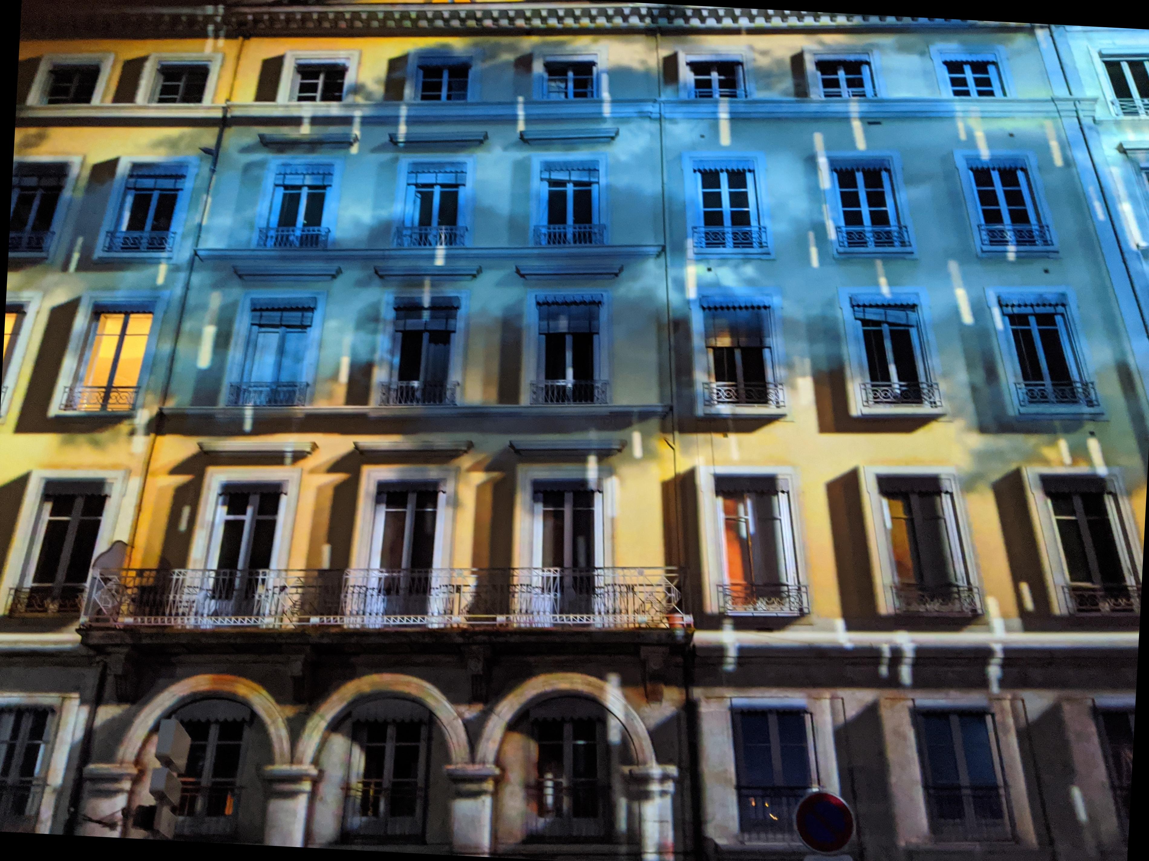
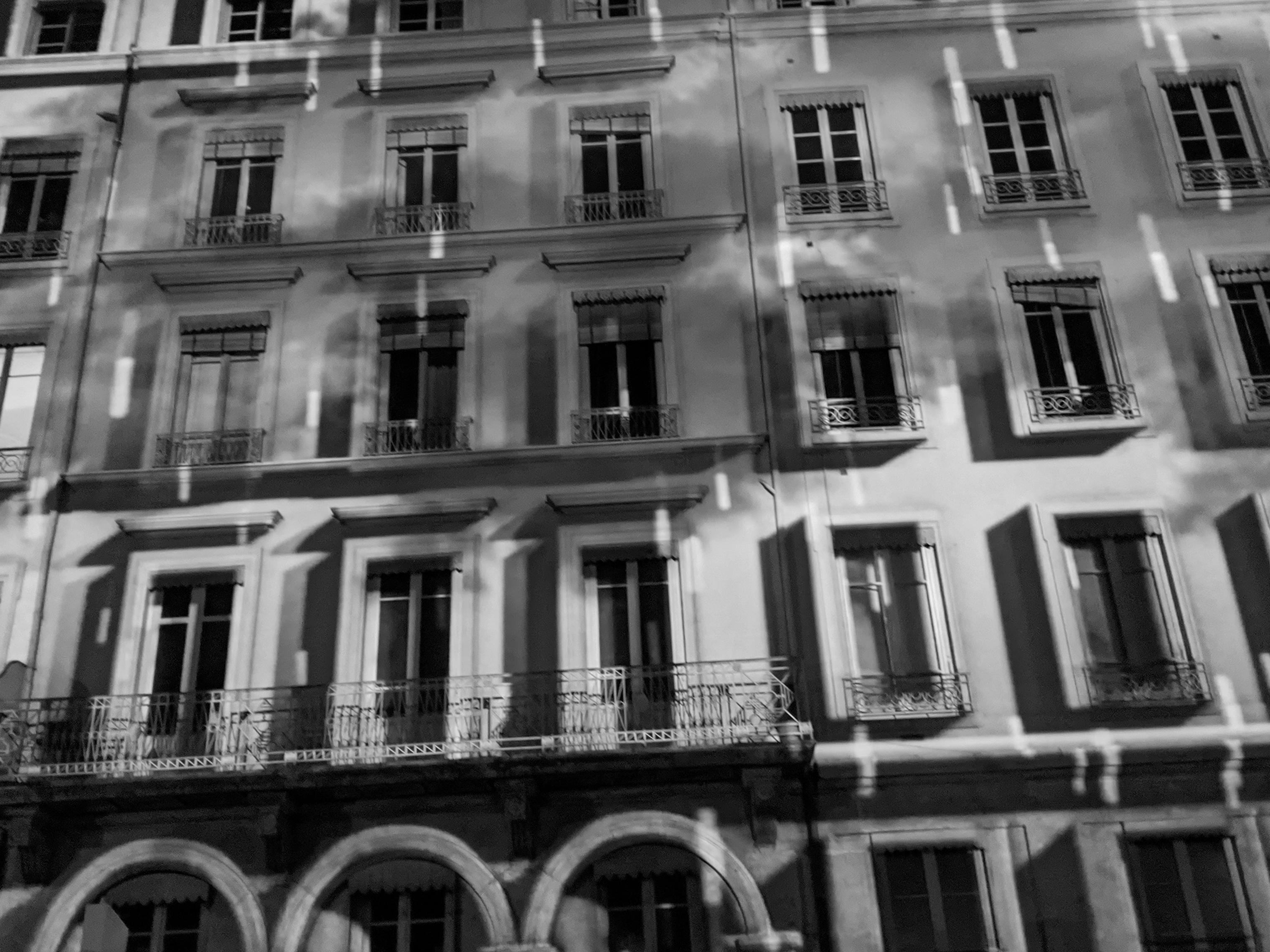
From the results above, i found that the final histogram is somewhat balanced. Then i tried the following images. It is obvious that if the scenery originally has more edges not in the horizonal and vertical orientation, the rotation matching effect would be bad.
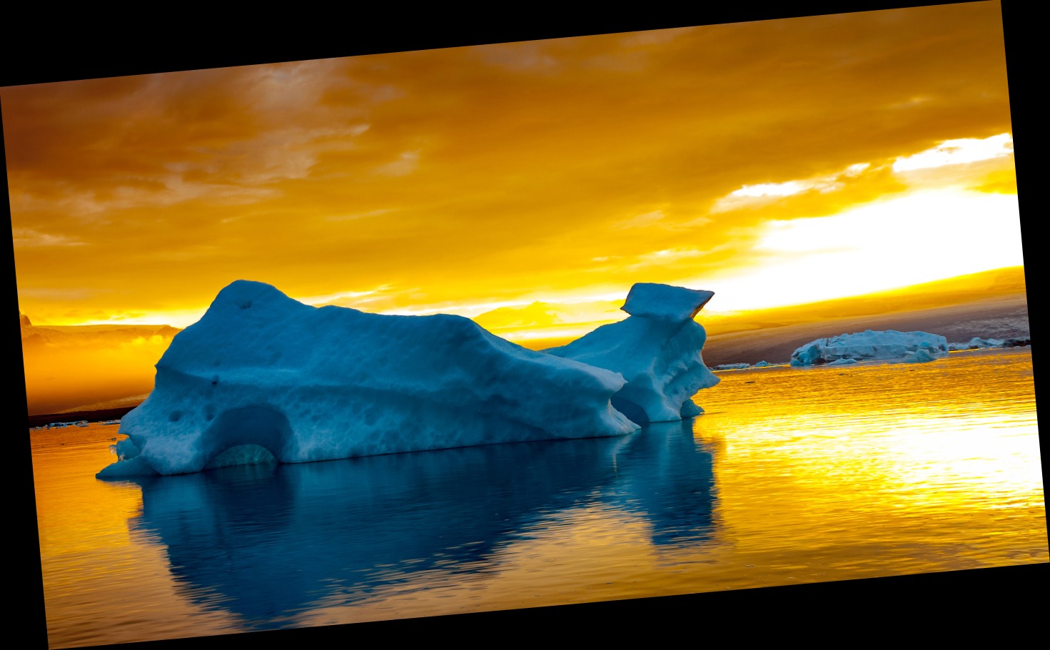 Ice_org
|
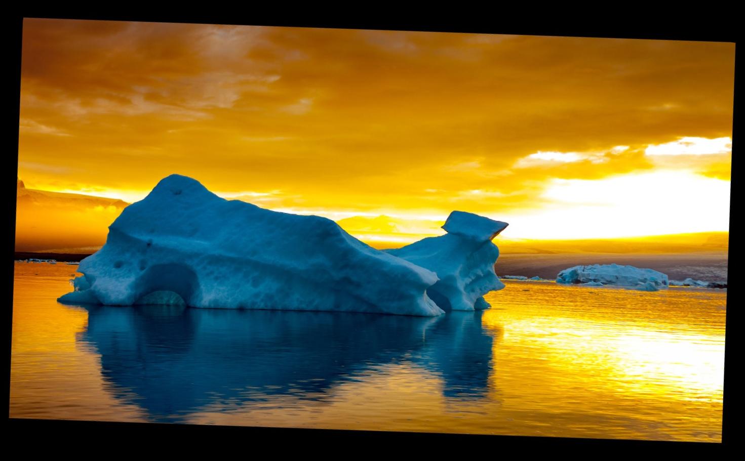 Ice_result(failed)
|
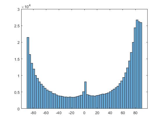 his_org
|
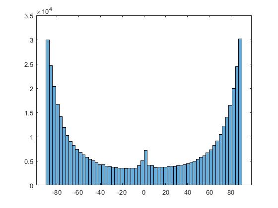 his_result
|
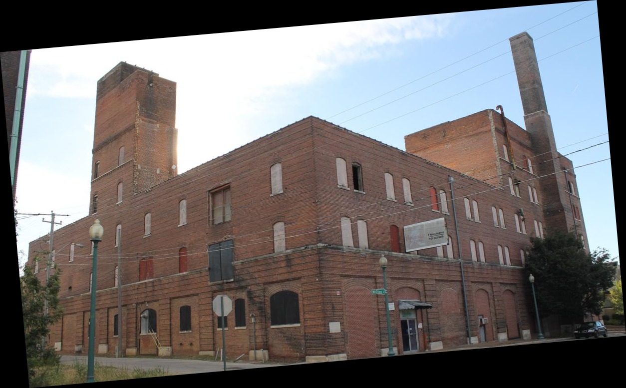 Build_org
|
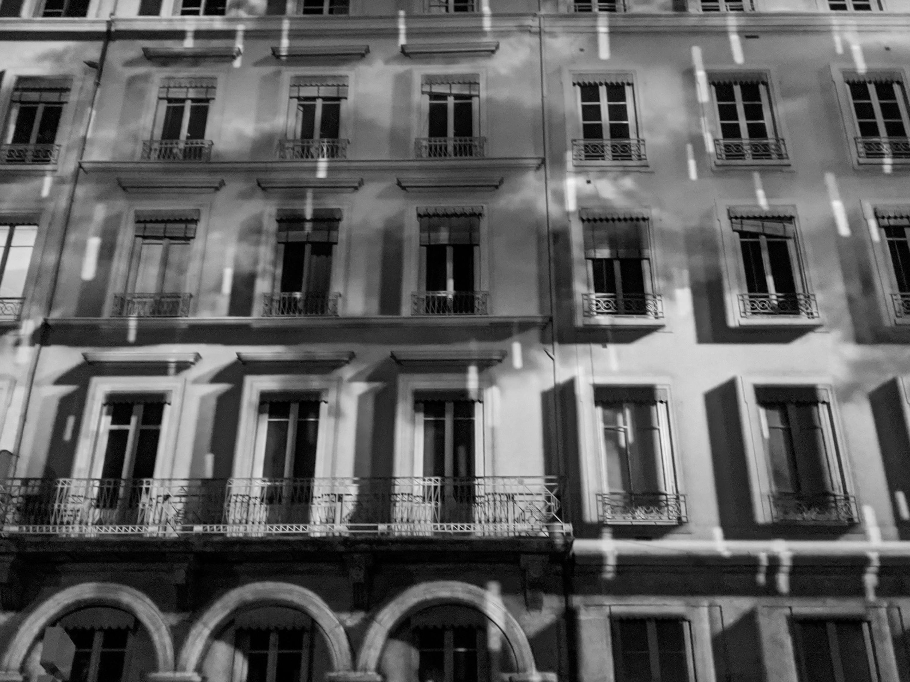
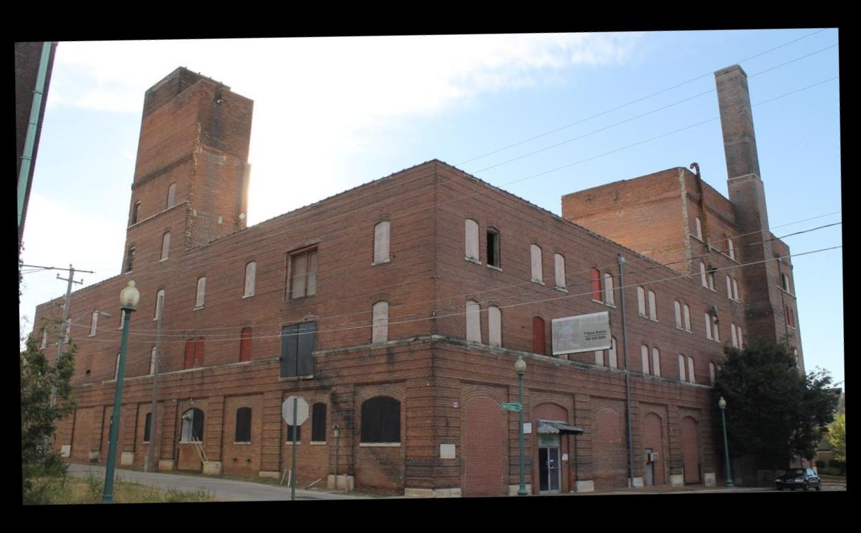 Build_result
|
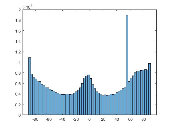 his_org
|
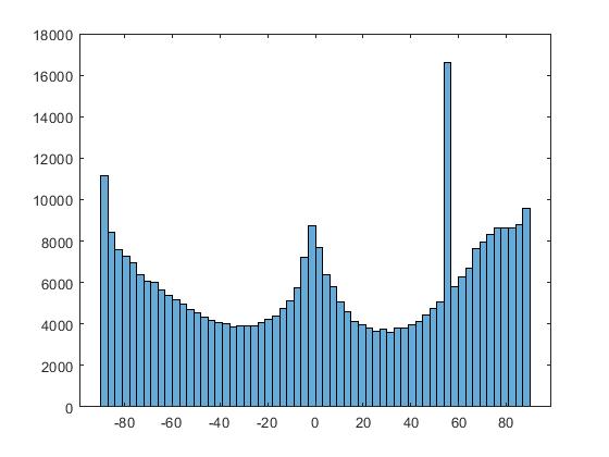 his_result
|
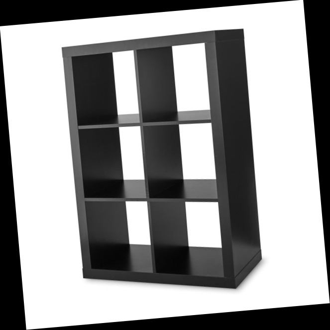 Shelf_org
|
 Shelf_result
|
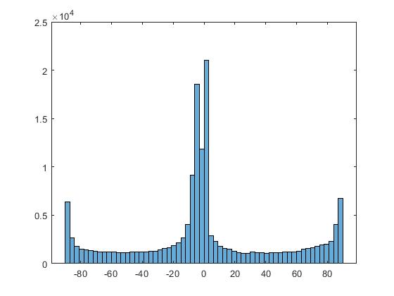 his_org
|
 his_result
|
Part 2: Fun with Frequencies!
2.1: Image "Sharpening"
High frequency part of image can be got when subtracting blurred version from the original image. Give a weight to the high frequency part and add it back to the original image, then the image is sharped. In order to make the above as a single process, we could do the convolution as following. Also I tried weight alpha = 2, 5 and 10. We could see that as weight increases, sharping effect is more significant.
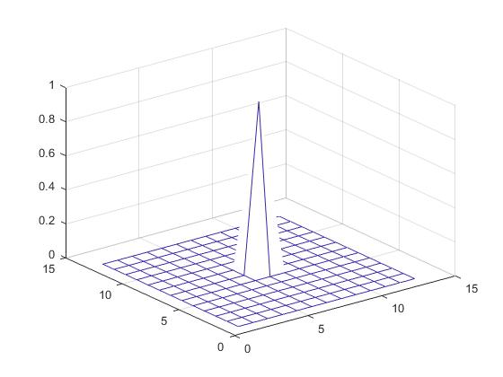 Unit impulse
|
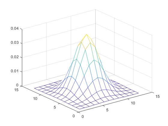 Gaussian
|
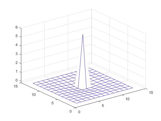 Laplacian of Gaussian
|
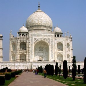 Org
Org
|
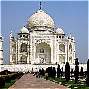 Alpha=2
|
 Alpha=5
|
 Alpha=10
|
 Org
Org
|
 Alpha=2
|
 Alpha=5
|
 Alpha=10
|
 Org
Org
|
 Alpha=2
|
 Alpha=5
|
 Alpha=10
|
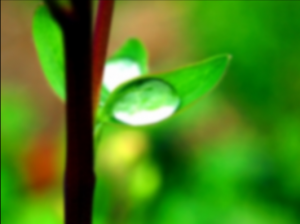
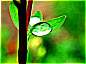
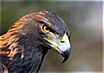
For the following, there is a sharp image of eagle. Then I used gaussian filter do the blurring. Finally, I followed the same process as the above to do the image sharpening. From the result, I found that after sharpening, the image is similar to the original one. But it cannot be the same as that. Because blurring is some kind of averaging and loss of information cannot be avoided. Sharpening also makes some unimportant features in the original image to be more significant.
 Org_sharp
|
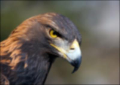 Blur
Blur
|
 Alpha=2
|
 Alpha=5
|
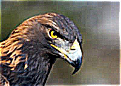 Alpha=10
|
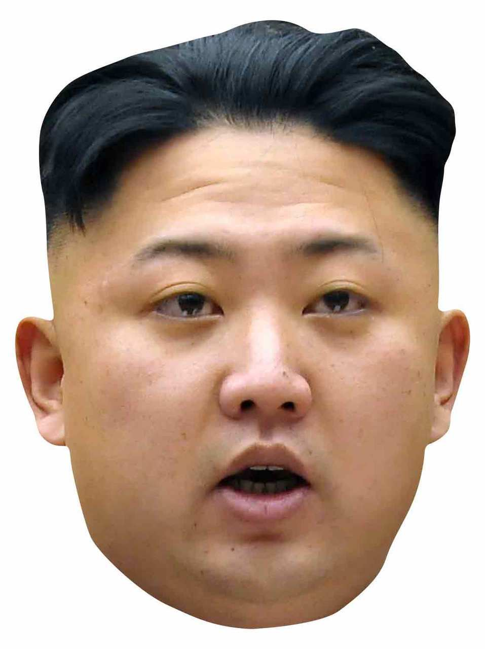
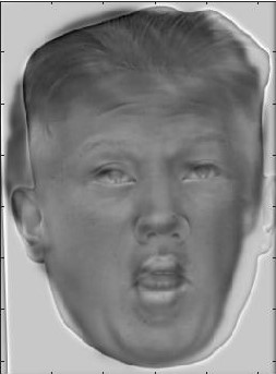
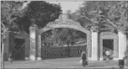
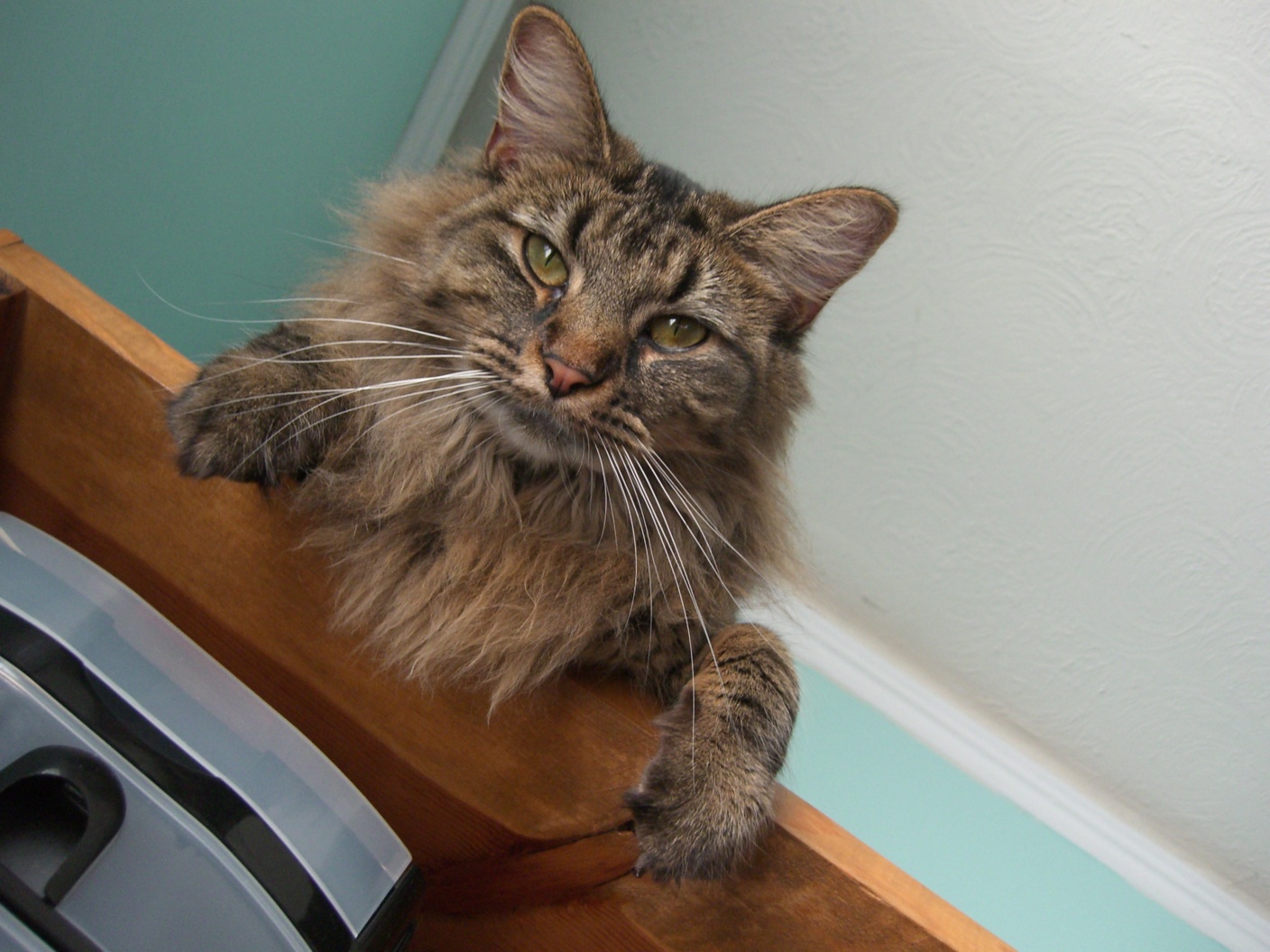
2.2: Hybrid Images
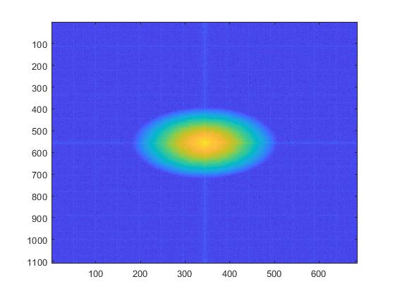
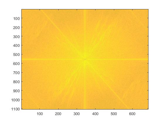
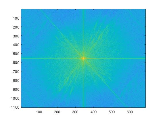
Low-pass filter used is Gaussian filter, and high-pass filter is impulse filter minus the Gaussian filter. Convolution in the original domain equals to multiplication in the frequency domain. So i convert low and high-pass filter to the frequency domain to process the image. After getting low and high frequency part of images, I just add them together to get the final hybrid image. Log magnitude plot of the Fourier transform of images are shown below. (Image alignment and cropping is done in the whole process)
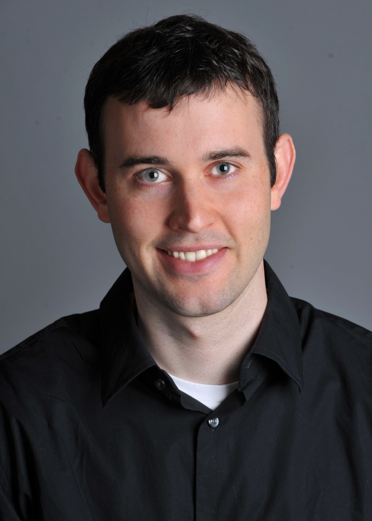 DerekPicture
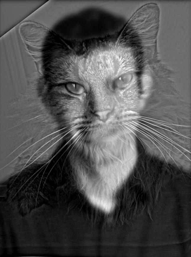
|
 Nutmeg
|
 Hybrid
|
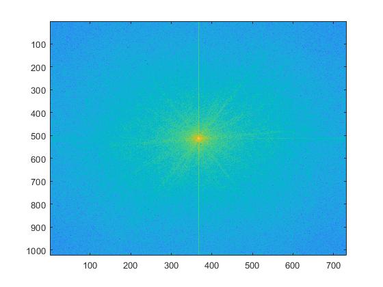 DerekPicture_fourier
|
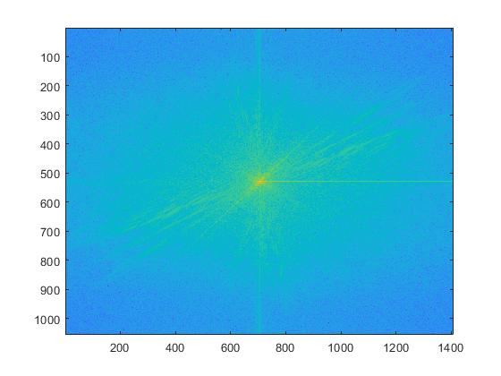 Nutmeg_fourier
|
 low_fourier
|
 high_fourier
|
 Hybrid_fourier
|
I also tried other images as following.
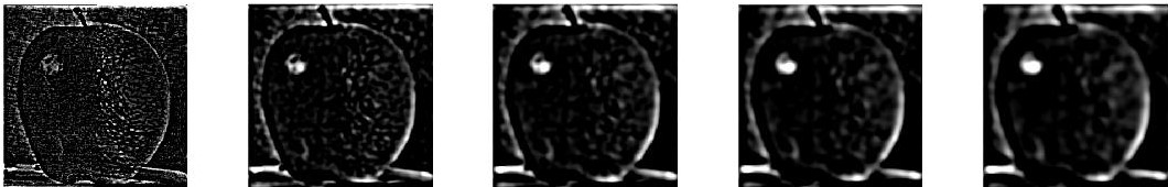
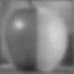
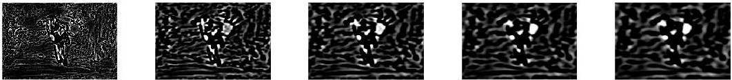
2.3: Gaussian and Laplacian Stacks
Stack is different from pyramid, which would not change the dimension of the image. Gaussian and Laplacian stack are similar. One is applying Gaussian filter in each step, and another is applying Laplacian of Gaussian filter in each step. I used matlab build-in method imadjust to make the residual significant enough for our eyes to see.
 Lincoln
|
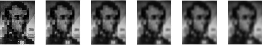 Gaussian stack
|
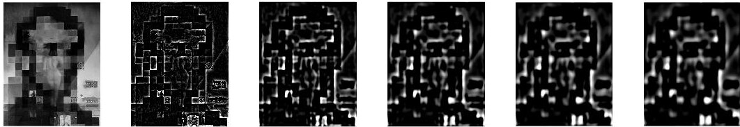 Laplacian stack
|
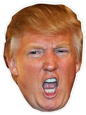
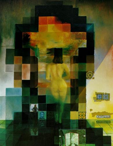
Then i applied Gaussian and Laplacian stack to the part 2.2's result. As we can see, in the part 2.2, i used Trump's low frequency part and Kim's high frequency part to get the hybrid image. Just check the first level of each stack, Trump becomes apparent in the Gaussian stack and Kim also becomes obvious in the Laplacian stack.
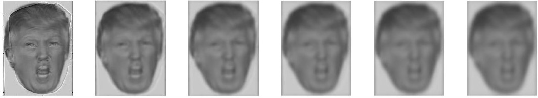 Gaussian stack
|
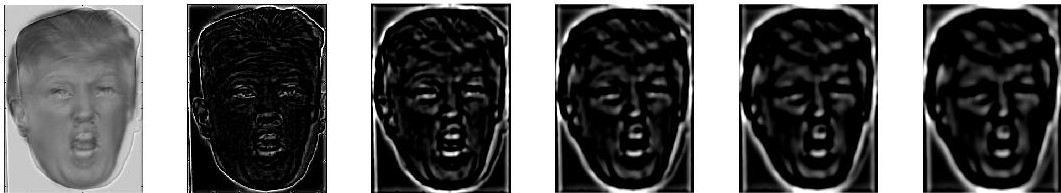 Laplacian stack
|
2.4: Multiresolution Blending
Here, my work is to combine two images with a smoothy seam. Then i used the algorithm mentioned in the 1983 paper by Burt and Adelson. Gaussian stack is applied to the mask image and Laplacian stack is applied to two input images in gray scale. Follow the algorithm and recontruct the blending image (LS+Blur). An oraple is got! I also showed blending effect directly using mask. We could see the obvious difference compared with the result.
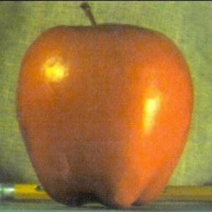 Apple
Apple
|
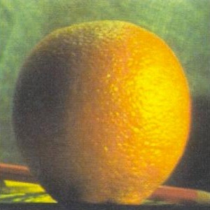 Orange
|
 Mask
Mask
|
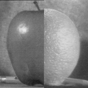 First_blend
|
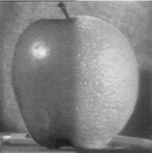 Result
|
 LS
LS
|
 Blur
Blur
|
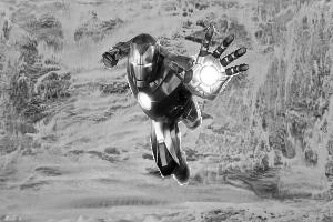
I also tried other images with irregular masks.
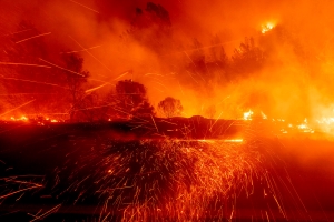 Fire
Fire
|
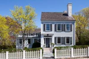 House
House
|
 Mask
Mask
|
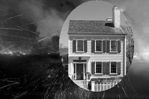 First_Blend
|
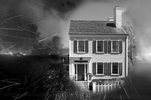 Blend
Blend
|
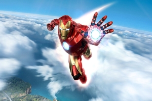 Ironman
|
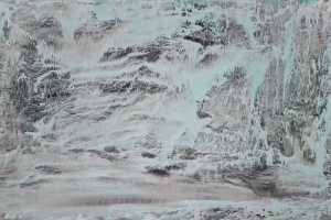 Shanshui
|
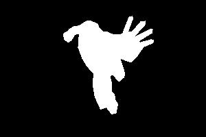 Mask
Mask
|
 First_Blend
|
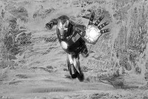 Blend
Blend
|
 LS
LS
|
References
[1] Oliva A, Torralba A, Schyns P G. Hybrid images[J]. ACM Transactions on Graphics (TOG), 2006, 25(3): 527-532.
[2] Burt P J, Adelson E H. A multiresolution spline with application to image mosaics[J]. ACM Transactions on Graphics (TOG), 1983, 2(4): 217-236.