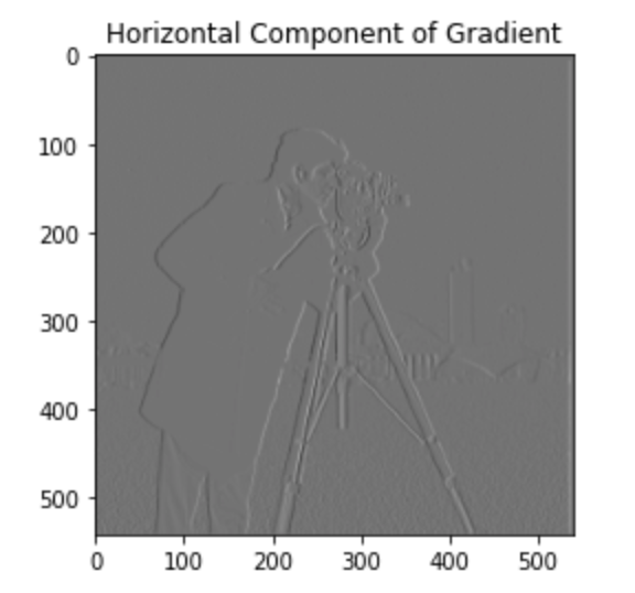
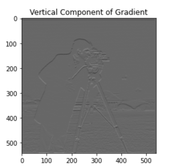
The purpose of this section is to explore image gradients. We set up two different kernels, the horizontal derivative kernel (D_x) and the vertical derivative kernel (D_y). To obtain the edge image we simply want to know how much the image is changing at a specific point, therefore we can compute the gradient of the gradient, where the gradient is the array containing D_x and D_y.
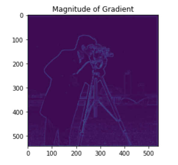
Specifically, the edge image is given by: E = sqrt(D_x^2 + D_y^2). Conceptually, at the pixel ( i,j) we have the magnitude of the gradient given by E_{ij}, but what if we want to know the direction of the gradient? We can easily compute that and store it in a matrix, T, where T_{ij} = arctan((D_y)_{ij}/(D_x)_{ij}).
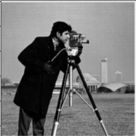
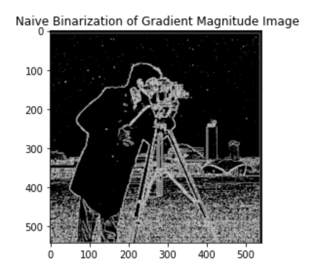
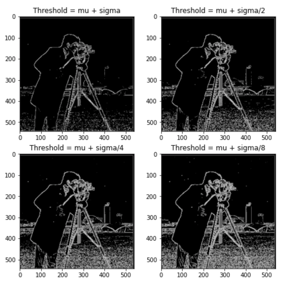
To make the edges more evident we binarize the magnitude of gradient image. This means we pick some threshold and set every value above the threshold to 1 and every value below the threshold to 0. The naive binarization algorithm takes the threshold equal to the mean pixel brightness. This works well but there is definitely room for improvement. From the last figure it seems that th = 𝜇+𝜎/2 is the best choice. Notice that although this seemed to be the best threshold it is still quite noisy. The grass patch makes it hard to get a proper edge image Here are the results of applying this on the cameraman image:
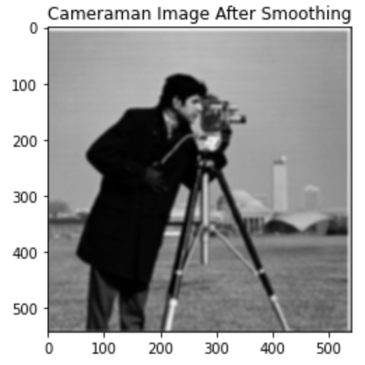
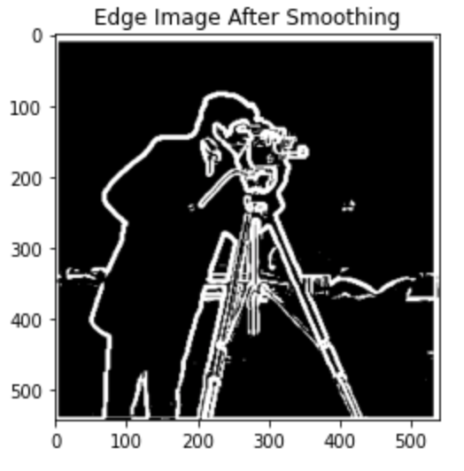
The issue with the naive edge image binarization was that the image is somewhat noisy, therefore we would like to blur the image before computing the edge image so that we get rid of the noise and get a cleaner edge image. Intuitively, noise is usually a high frequency component of the image since it involves small fluctuation in nearby pixels. Therefore, by applying a gaussian blur we are effectlively applying a low pass filter to the image which gets rid of these high frequency fluctuations.
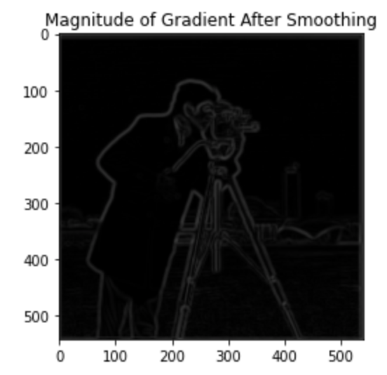
We first smooth the image with a size 7 gaussian kernel and then perform the same operations outlined in the previous section. Here are the results:
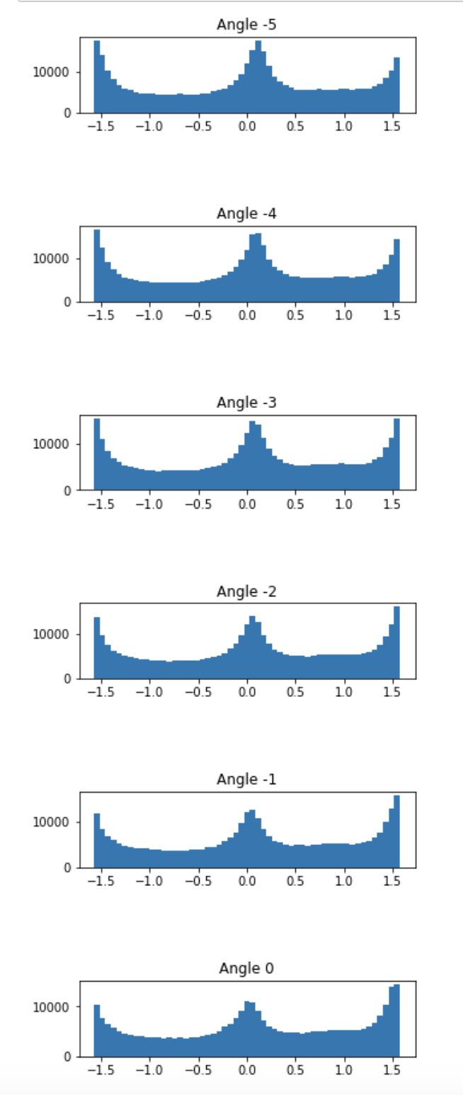
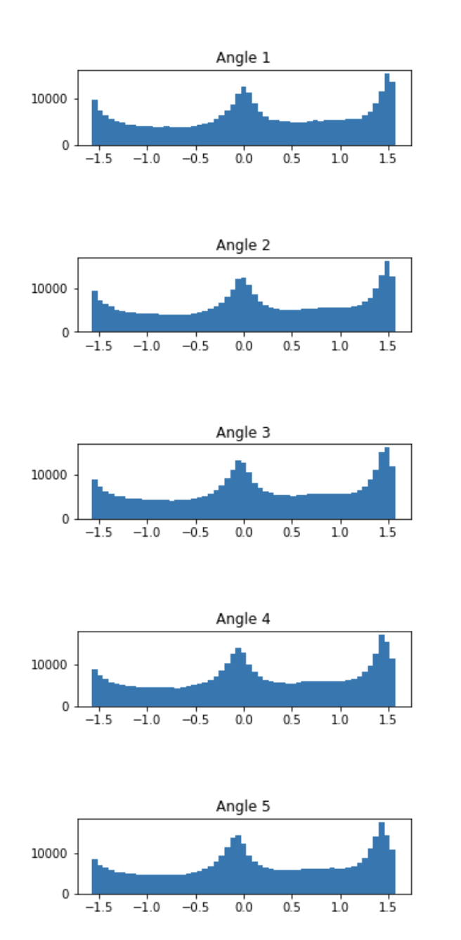
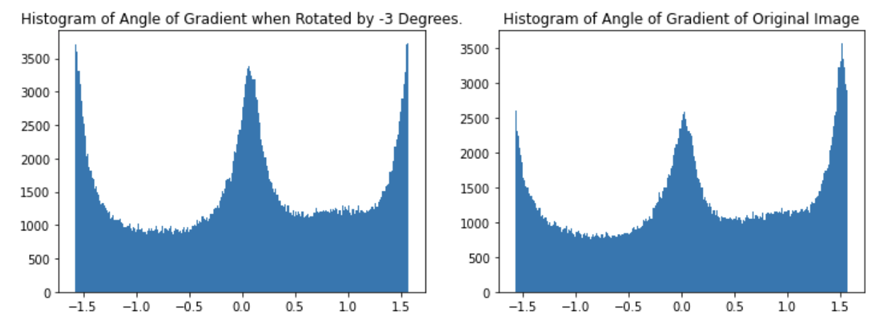
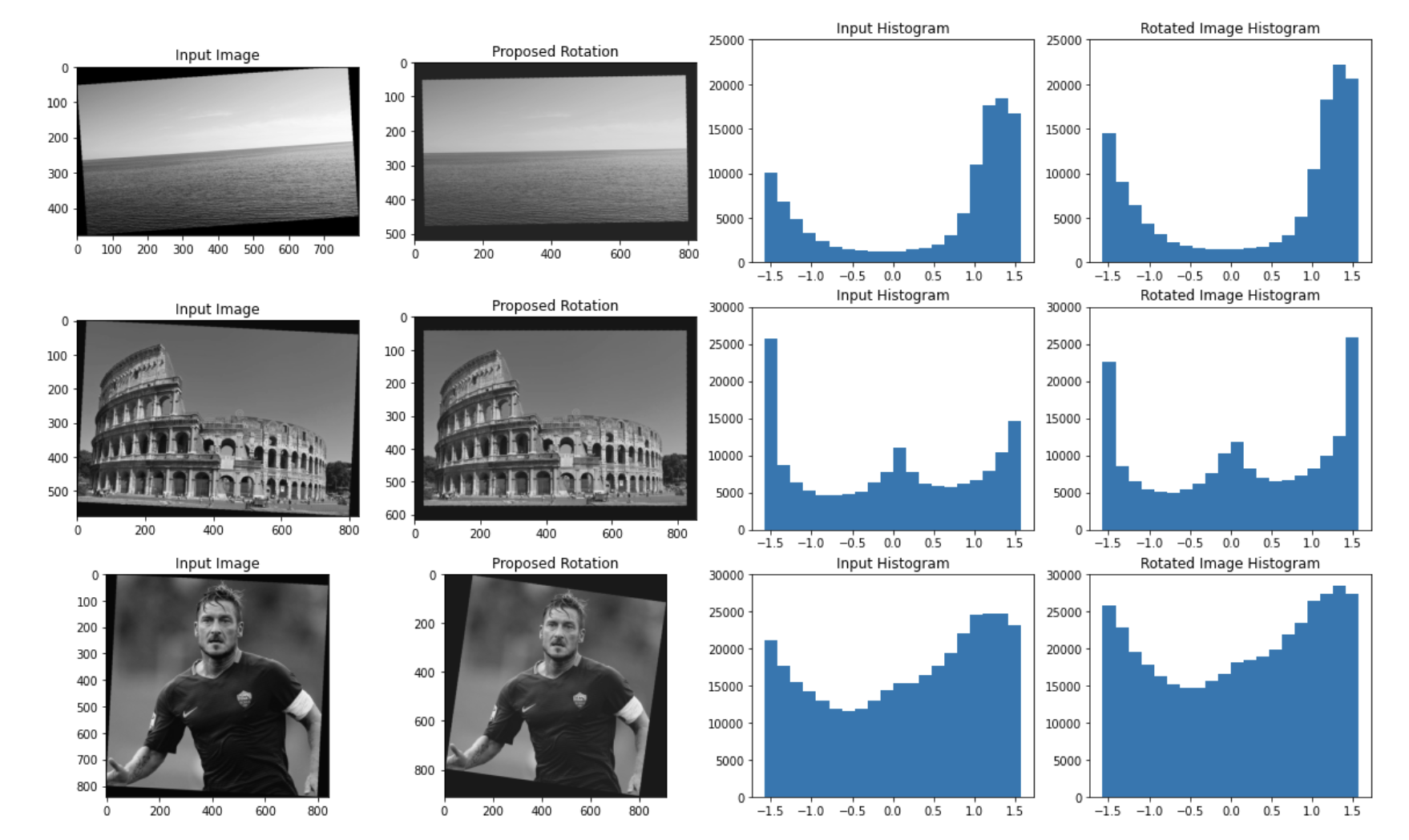
In this section we explroe algorithms to automatically align images. The idea is that we can compute the edge image for a given image and then look at the angle image. The process to obtain the angle image, T, was described in section 1.1. Once we have the angle image we can plot a histogram of values, in theory most pictures should have vertical edges because gravity acts vertically. We will see that this assumption works well on most pictures.
My algorithm works as follows: first obtain the angle image, then plot the histogram of angle values. I then pass this into a function and solve the following optimization problem: argmin_i abs(# of entries in -pi/2 bucket - # of entries in pi/2 bucket) - eps*w1 - eps*w2
Here i is a rotation of the image which loosely translates to a shift in the histogram, w1 = max(pi/2 bucket, -pi/2 bucket)*min(-pi/2 bucket,pi/2 bucket) and w2 = 0 bucket. Breaking it down the intuition is that ideally the historgam of an aligned image should have three peaks, at -pi/2, pi/2 and 0. Since these correspond to vertical and horizontal edeges, respectively. Therefore the absolute difference makes sure that the peak at pi/2 is more or less the same height as the peak at -pi/2. Since this could be minimized when they are both close to zero we add w1, this is lower the higher the peaks are, finally w2 is subtracted to make sure that we also take into account the number of entries in the 0 bucket and account for horizontal edges.
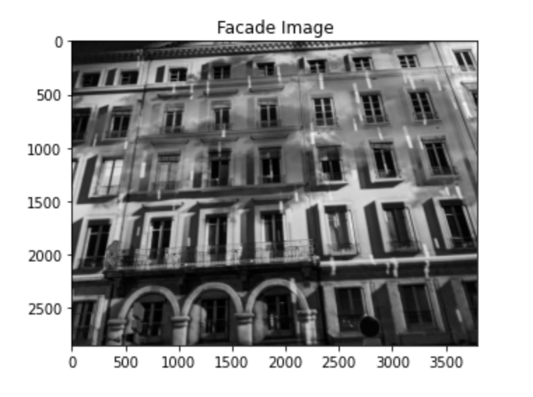
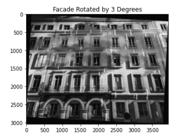
Here we will present the input facade image, the various histograms, and the proposed rotation by my algorithm.
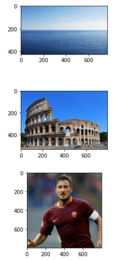
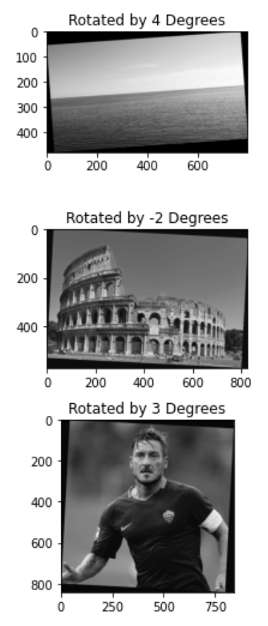
Here is my result when I ran it on three different images:
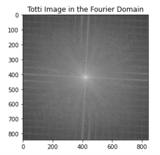
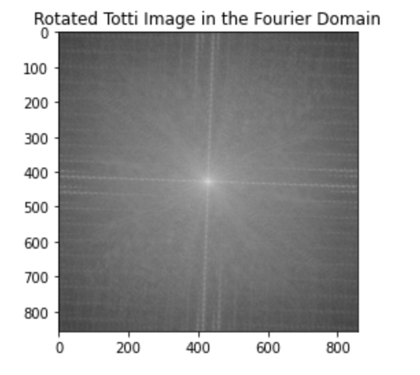
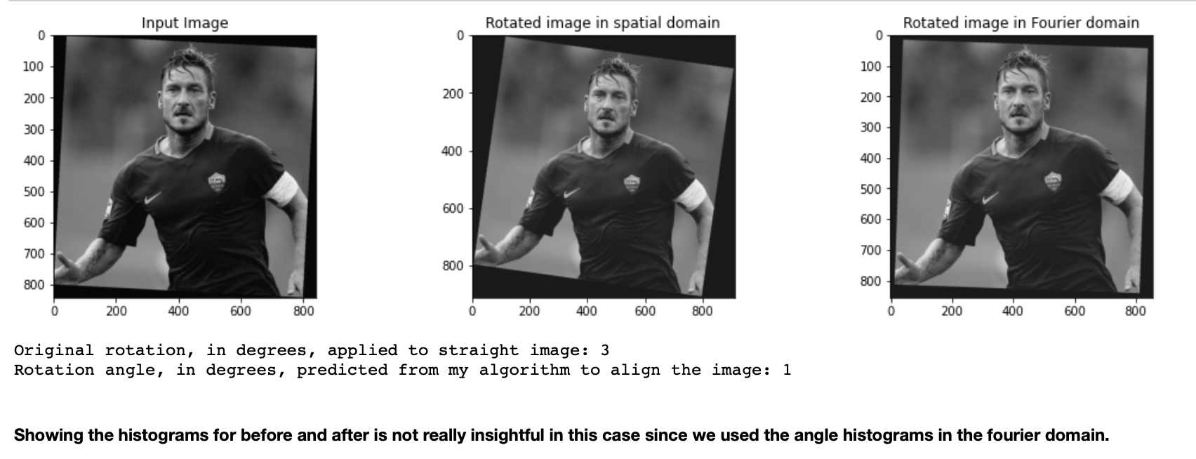
As we saw in the previous section, some images can't be properly aligned. Therefore we perform the alignment in the fourier domain. Here we show the input image in the fourier domain, and then the result after applying the rotating algorithm in the fourier domain.
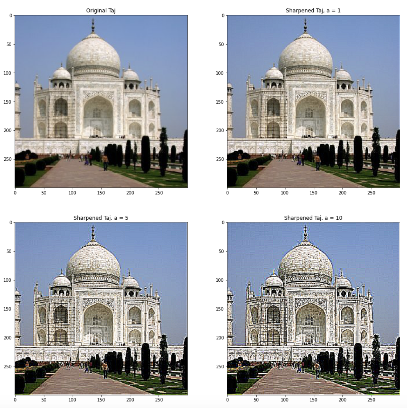
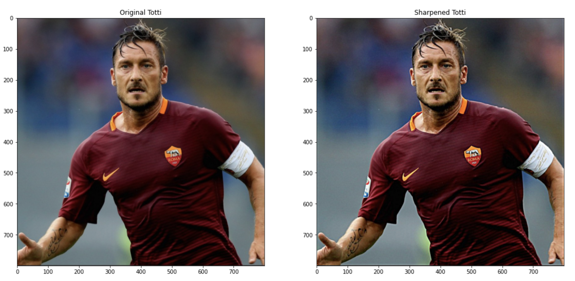
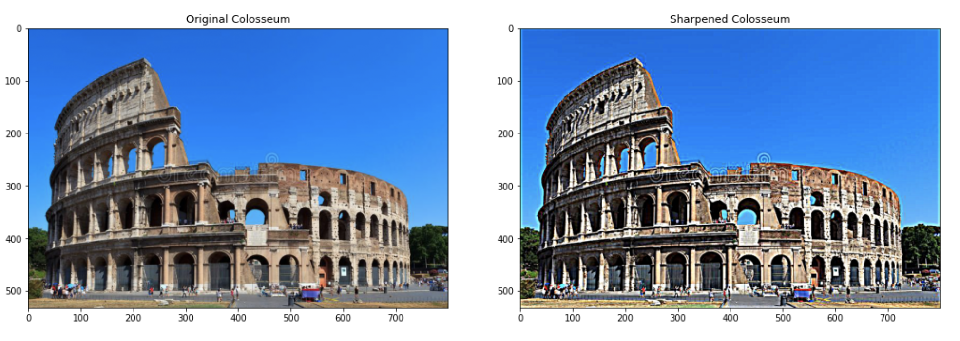
In this section we explore image sharpening. I created a filter that automatically sharpens an image. To sharpen an image we want to add the high frequency components of the image so that we emphasize these. Intuitively, to obtain the high frequency components we can convolve the input image with F = (d - G), where d is the 2d kronecker delta signal (0's everywhere except in the center pixel where it equals 1), and G is the gaussian filter. This will give us a high pass filter. We then want to add this back into our image, therefore we want to convolve our image with (d + aF), where a is a sharpening coefficient that will determine how strong our sharpness is. Putting all this together we get our sharpening filter S = d + ad - aG = d(a+1) - aG. Doing this we can sharpen the image with one convolution. Here are some results using a 13x13 gaussian filter with sigma = 5:
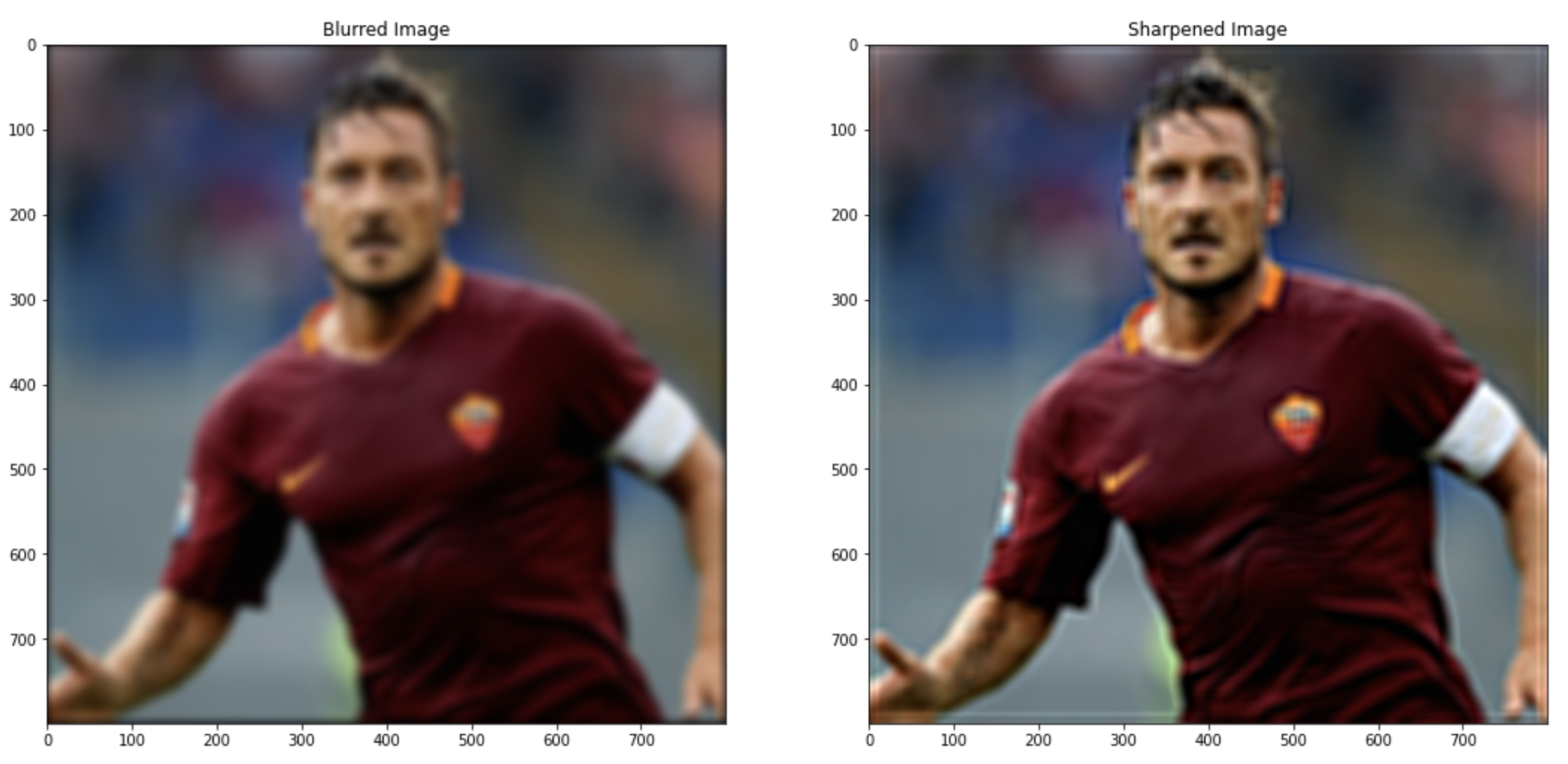
Another interesting thing I tried was to blur an image beforehand using a gaussian filter of size 21 with sigma = 7, and the sharpening it. We see that it doesn't work too well. This is because when we blur an image we effectively remove the high frequency components of the image, so even when we add back the high frequency components it doesn't work because there aren't high frequency components to begin with! We also need to provide a really big coefficient to the function which results in a blurry image with somewhat defined edges. Notice that although it's not a pretty picture we can see Totti's lips and eyebrows whereas in the blurred image its hard to make out the details. Here are the results:
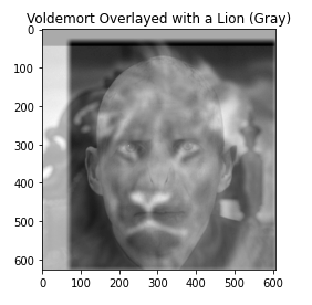
The goal of this task is to create an algorithm that creates hybrid images as described by the 2006 SIGGRAPH paper by Oliva, Torralba, and Schyns. As described in the spec:
Hybrid images are static images that change in interpretation as a function of the viewing distance. The basic idea is that high frequency tends to dominate perception when it is available, but, at a distance, only the low frequency (smooth) part of the signal can be seen. By blending the high frequency portion of one image with the low-frequency portion of another, you get a hybrid image that leads to different interpretations at different distances.
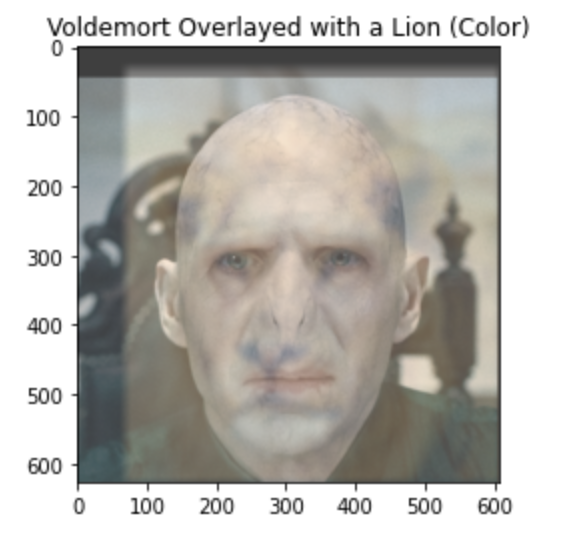
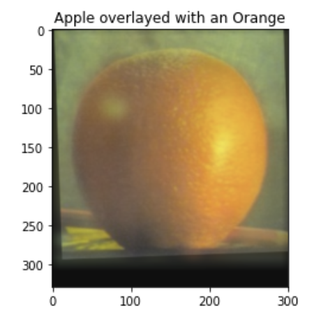
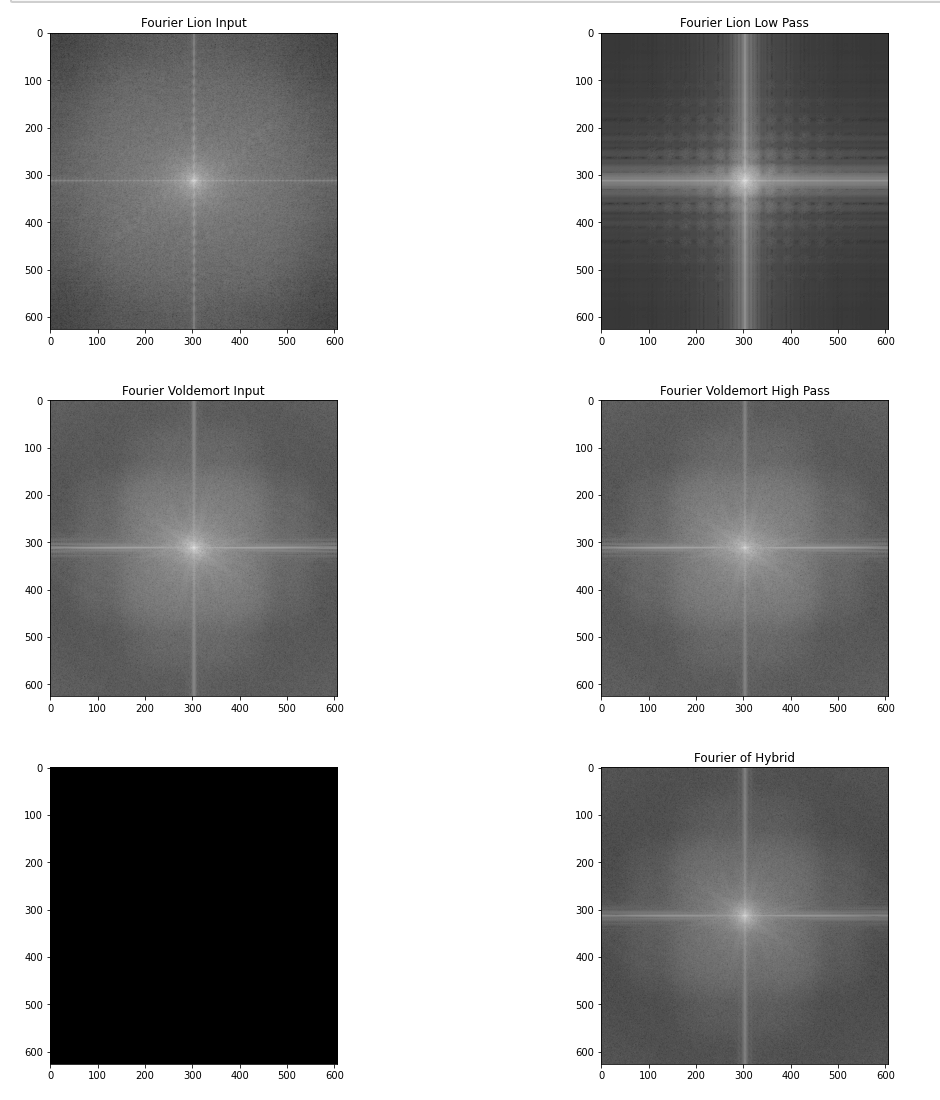
The algorithm is very simple and leverages functions from the previous parts, we convolve im1 with F, a high pass filter as described in the previous tasks, and we convolve im2 with G, a low pass filter. Both kernels have size 17x17, the low pass filter has a sigma of 11 since we want a sharp cutoff frequency, this is inversely proportional to the sigma as it appears in the denominator of the gaussian. Here are some results, it seems to work well both in color and grayscale.
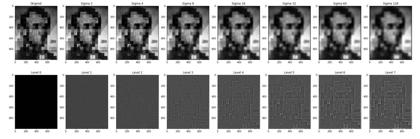
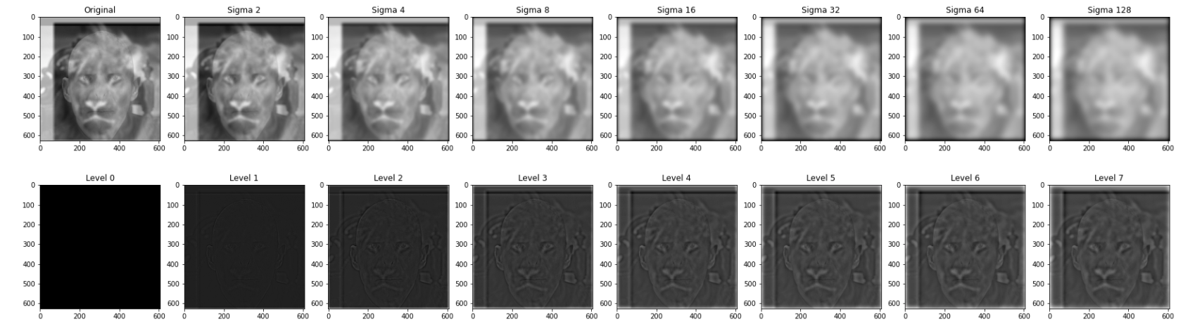
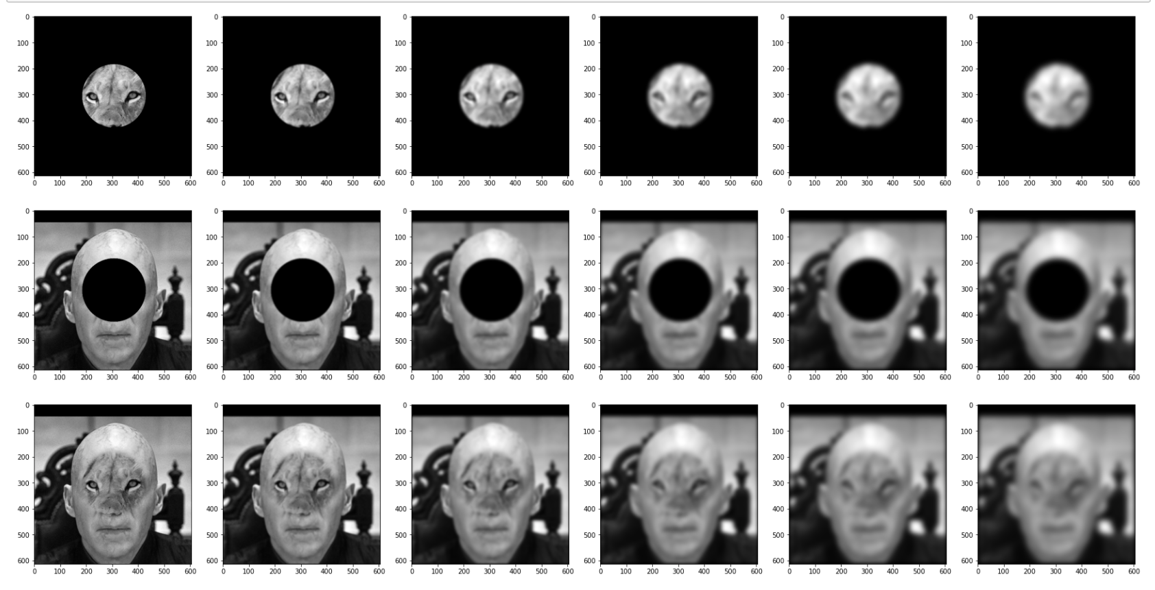
In this section we implement gaussian and laplacian stacks. In gaussian stack we simply apply a gaussian blur at each step with an increasing sigma value so as to make the low pass filter more and more sharp. At each level of the stack I double the sigma value. The laplacian stack is built by taking the difference between the original image and the gaussian stack at each level. Intuitively, the laplacian stack is a stack at which each level we keep higher and higher frequency components, this is the exact opposite of the gaussian stack.
Here are some examples:
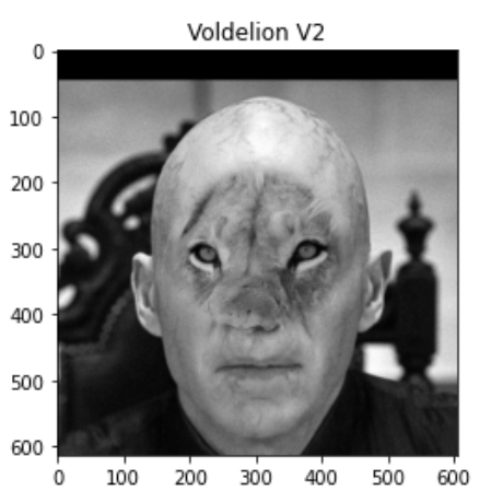
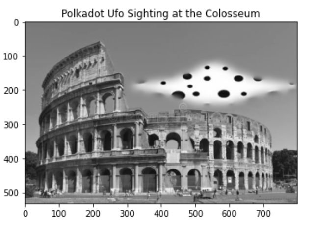
In this section we implement the multiresolution blending as described in the 1983 paper by Burt and Adelson. Multiresolution blending computes a gentle seam between the two images seperately at each band of image frequencies, resulting in a much smoother seam. We begin by creating a mask and its gaussian stack, and gaussian and laplacian stacks for the images.
We then blend the images by creating a stack of images in which every image at level k is given by: (I_k)_{ij} = (Lalplacian_k(im1))*(Gaussian_k(mask))_{ij} - (Lalplacian_k(im2))*(1 -Gaussian_k(mask))_{ij}. To get the original image we then add the stack in the blended image. Why does this work? Intuitively every image is composed of very different bands of frequencies, this method achieves a good blending because we blend the image at different frequency values and then add them back together. Here are some examples:
In this project I learned a lot, it definitely gave me a deeper understanding of how geometrical shapes in the spatial domain affect the fourier domain. I also really enjoyed the blending of images, I understand the importance of blurring to remove noise and adding elements in various frequency domains to obtain nicer and cleaner results.