Project 2: Fun with Frequencies and Filters!

For the second project of the Introduction to Computer Vision and Computational Photography, we were tasked with messing around with photos to learn some basic cv functions.

Project Overview

We had a lot of freedom with this project as long as we provided the desired images for the project overall.

Part 1: Fun with Filters

In this part, we will build intuitions about 2D convolutions and filtering. So, here's where we got to play with some filters.

Part 1.1

We will begin by using the humble finite difference as our filter in the x and y directions. First, I convolve my image with the finite difference operators: 𝐷𝑥=[1−1] 𝐷𝑦=[1−1]^T

Here is the original photo:

This results in the x and y-derivatives of the image:

Then, I used the 𝐷𝑥 and 𝐷y images to get the gradient magnitude image by using the formula: magnitude = sqrt(𝐷𝑥^2 + 𝐷y^2). I then binarized the image(everything above a certain threshold of .24 was set to 1, while everything below that threshold became 0). That resulted in this image:

Part 1.2

The image produced in part 1.1 has results that were particularly noisy, so in part 1.2, I will be using a low-pass Gaussian filter to hopefully get a better edge image.

I used a Gaussian filter of size 7 by 7 with a sigma value of 2.4. First, I convolved the original image with partial derivatives in x and y like before. Them I convolved that output with this Gaussian filter to get a blurrier/smoothed version of the original cameraman.png image. Afterward, I produced this edge image with a threshold of 0.2:

Part 1.3

Here was a part of the project I had the most trouble with, but still succeeded. I, like many, sometimes take a really nice photo but it's a little off-center. In this part of the project, we were tasked with creating an automatic straightening function.

For this I,

1. Rotate the image by a degree of 1 (through a specific range both in the left and right direction)
2. Crop the image so the center is just showing to avoid edges created by rotating the image
3. Compute the gradient angle of the edges in the image, by firstly getting the derivative in the x and y directions
4. compute the angle of the edge using the following formula: angle = arctan2(dy/dx);
5. Create a histogram of these values
6. Inspect the histogram to find the angle range around increments of 90 degrees as we can approximate these as "straight vertical and horizontal edges"
7. Pick the image with the highest number of straight edges.

Here is the successful image case of automatic straightening:

Because the first photo is taken at an angle, and the second photo has the subject naturally at an angle, they are not intended to be seen as straightened photos.

Part 2: Fun with Frequencies

Part 2.1

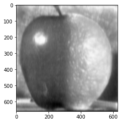
For this part of the project, we were tasked with sharpening blurry images. I convolved the image with the Gaussian filter once again to get a blurry image. Then I subtracted the blurry image for the regular one to get high frequencies and scaled it with an alpha to get a sharpened image. Here are some photos:

Here is where I took an already sharp image, blurred it, and then tried to sharpen it again. As you can see, some details are lost in the blurring of the image.

Part 2.2

For this part of the project, I had to create hybrid images using the approach described in the SIGGRAPH 2006 paper by Oliva, Torralba, and Schyns. Hybrid images are static images that change in interpretation as a function of the viewing distance. By blending the high-frequency portion of one image with the low-frequency portion of another, you get a hybrid image that leads to different interpretations at different distances.

For this I have some results:

This case didn't work out too well:

Part 2.3

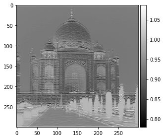
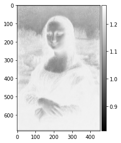
In this part, I had to implement gaussian and laplacian stacks. Below you can see how the images changes each time a gaussian or laplacian filter is applied:

Part 2.4

For the final portion of the project, we were required to do the multiresolution blending. I created a mask and then applied a Gaussian filter on it. I then applied Laplacian filters on the images and the Gaussian filter on every level on the stack. Then I added the images together and we get a multiresolution blend of the two images.

Final Thoughts

Why did this project break me? I mean, it was sorta fun, but I ran into so many troubles and obstacles throughout. I would be lying if I said I did not cry while completing this. I am very proud of the outcome, but I do not think I had too much fun. I am excited to learn more about hybrid images and face morphing in the next few weeks in our class. Overall, super-tough project with a bit of buggy code, but they say warriors are made in the midst of trials. I would not call myself a warrior either, but I am on my way.