Fun With Filters and Frequencies!

1. Fun with Filters
2. Fun with Frequencies!
3. Interesting Project Aspects

In this project, we played with different kinds of filters to manipulate images and separate high and low frequencies.

1 Fun with Filters

1.1 Finite Difference Operator

This filter uses the finite differences between the x and y directions to get a gradient magnitude image. We convolve the original image with two finite difference operator, Dx = [1 -1], Dy = [1 -1]^T. As a result, the original image is turned into an edge image.

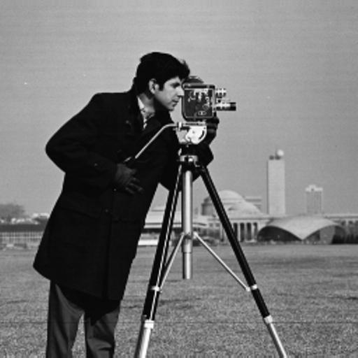
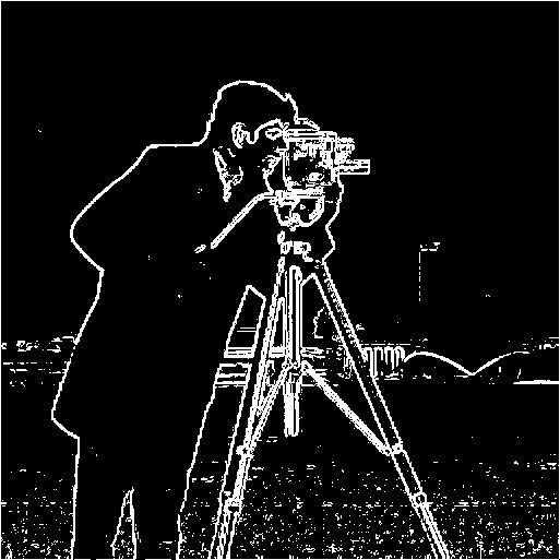
The result with the difference operator is really noisy. We further deduce the noise by using a Gaussian filter.

1.2 Derivative of Gaussian (DoG) Filter

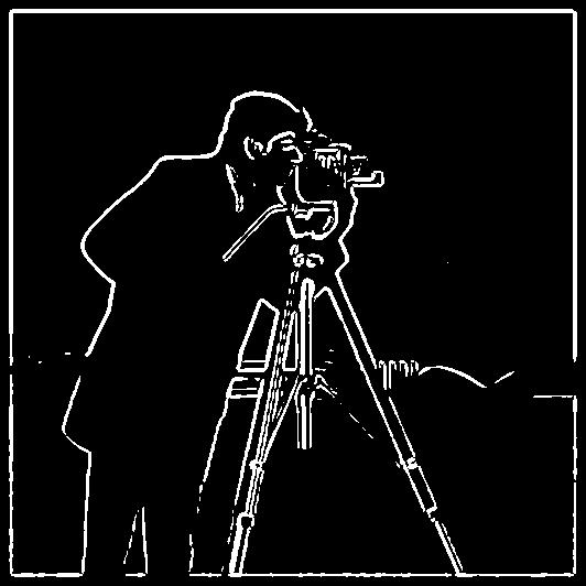
In order to remove the noise, we use a Gaussian filter. We convolve the original image with a Gaussian filter. The way to create a 2D gaussian filter is by using cv2.getGaussianKernel() to create a 1D gaussian and then taking an outer product with its transpose to get a 2D gaussian kernel. We can do the same thing with a single convolution instead of two by creating a derivative of gaussian filters. The borders are smoother and the noise is gone since the Gaussian filter removes the high frequencies.
The result is shown below.

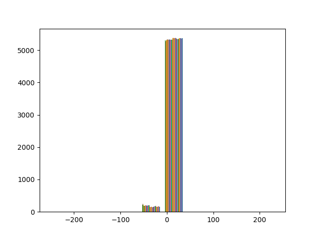
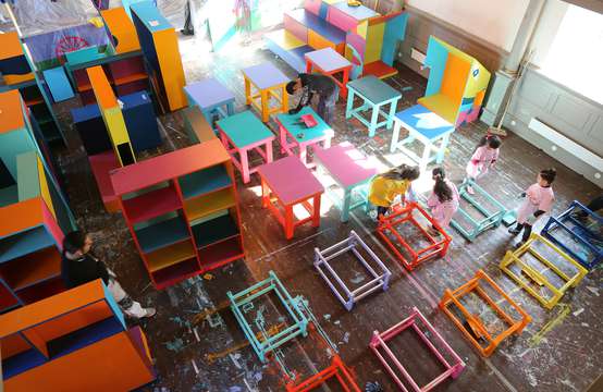
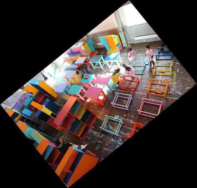
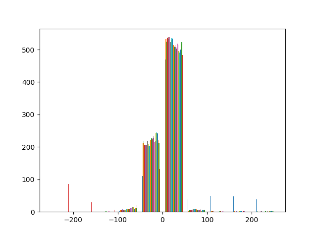
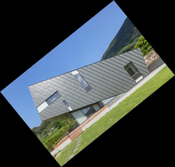
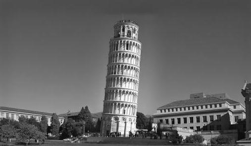
1.3 Image Straightening

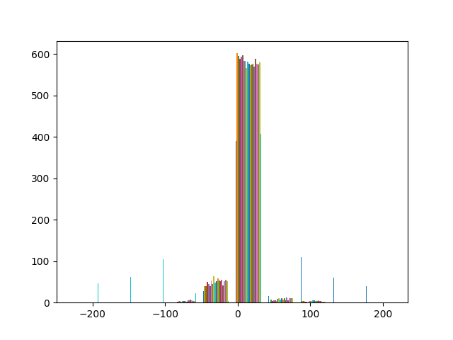
Sometimes the images we take are not straight. To straighten an image, we can use the derivative map to find perpendicular angles to the axis. We find the rotation angles with the maximum number of horizontal and vertical lines. Additionally, we need to crop the image in order to process only the actual image content. I divide the image by 5 and process it this way. The range of angles of my searching is [80, ..., 100] degrees. The results are shown below.

→

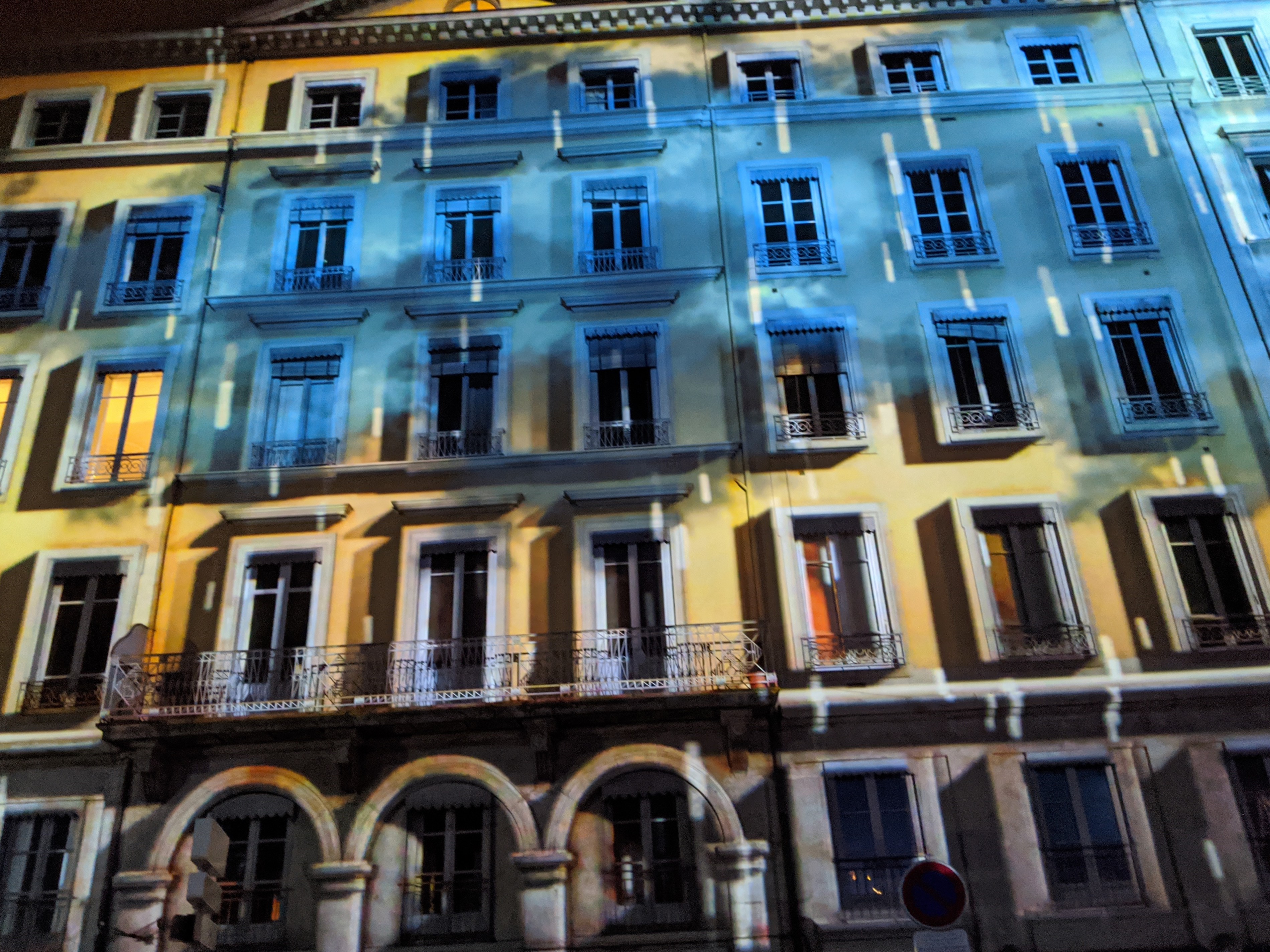
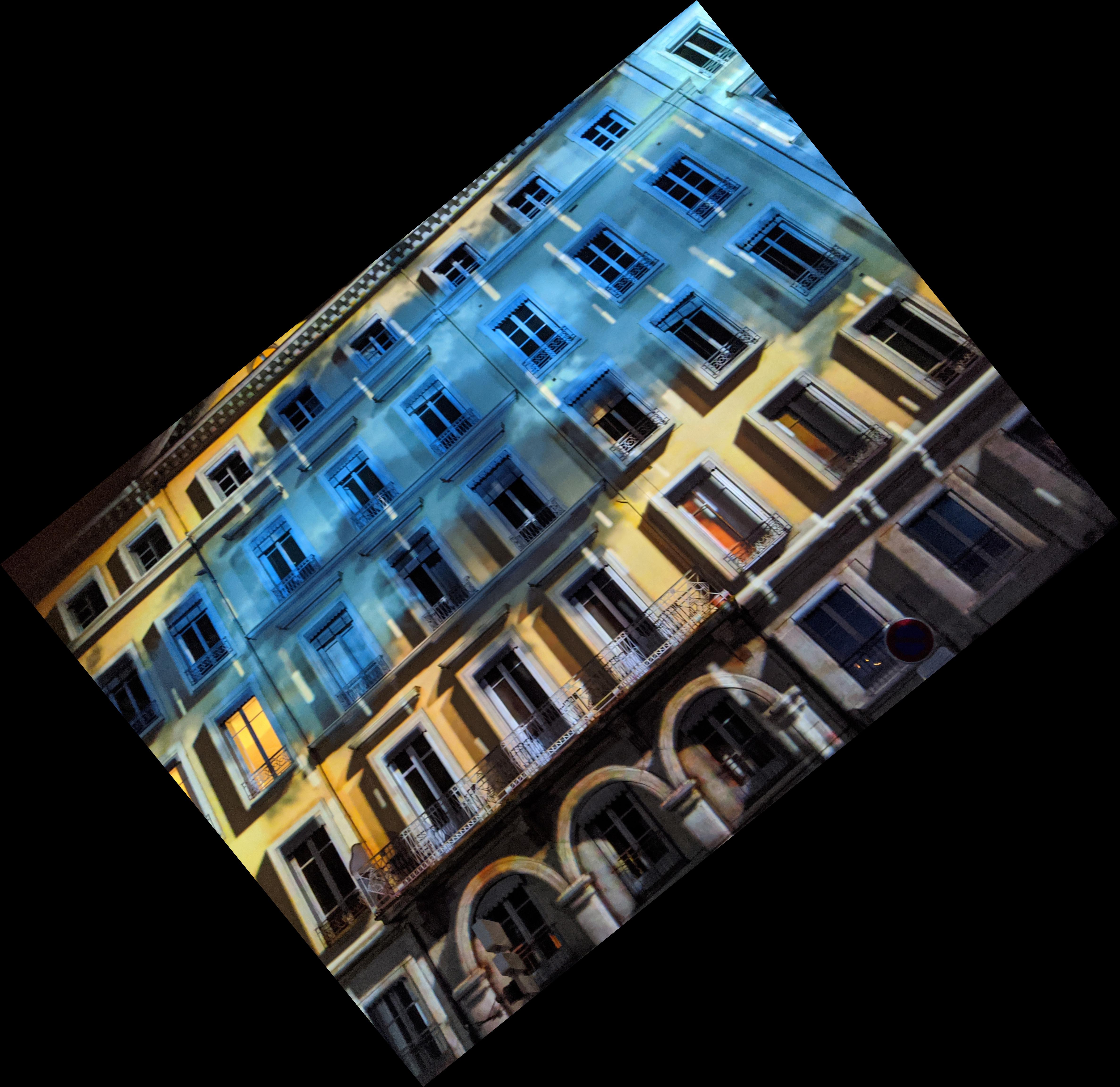
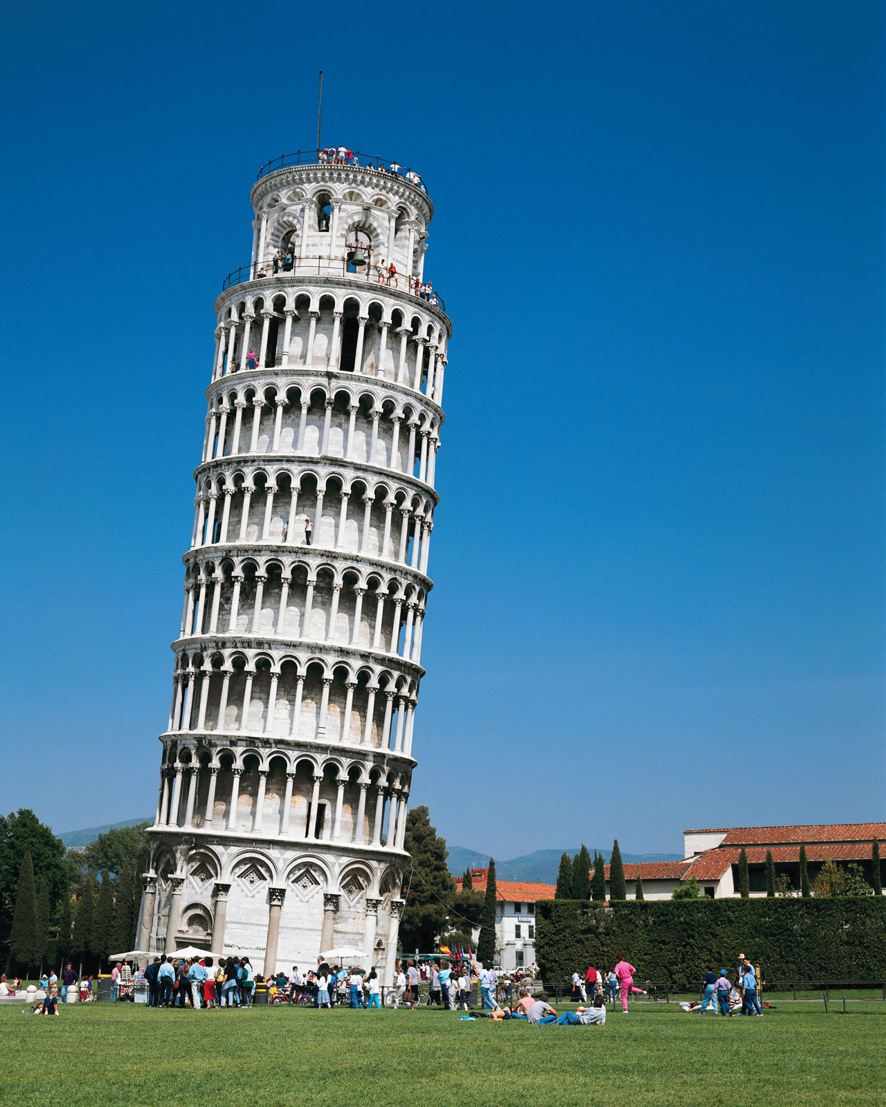
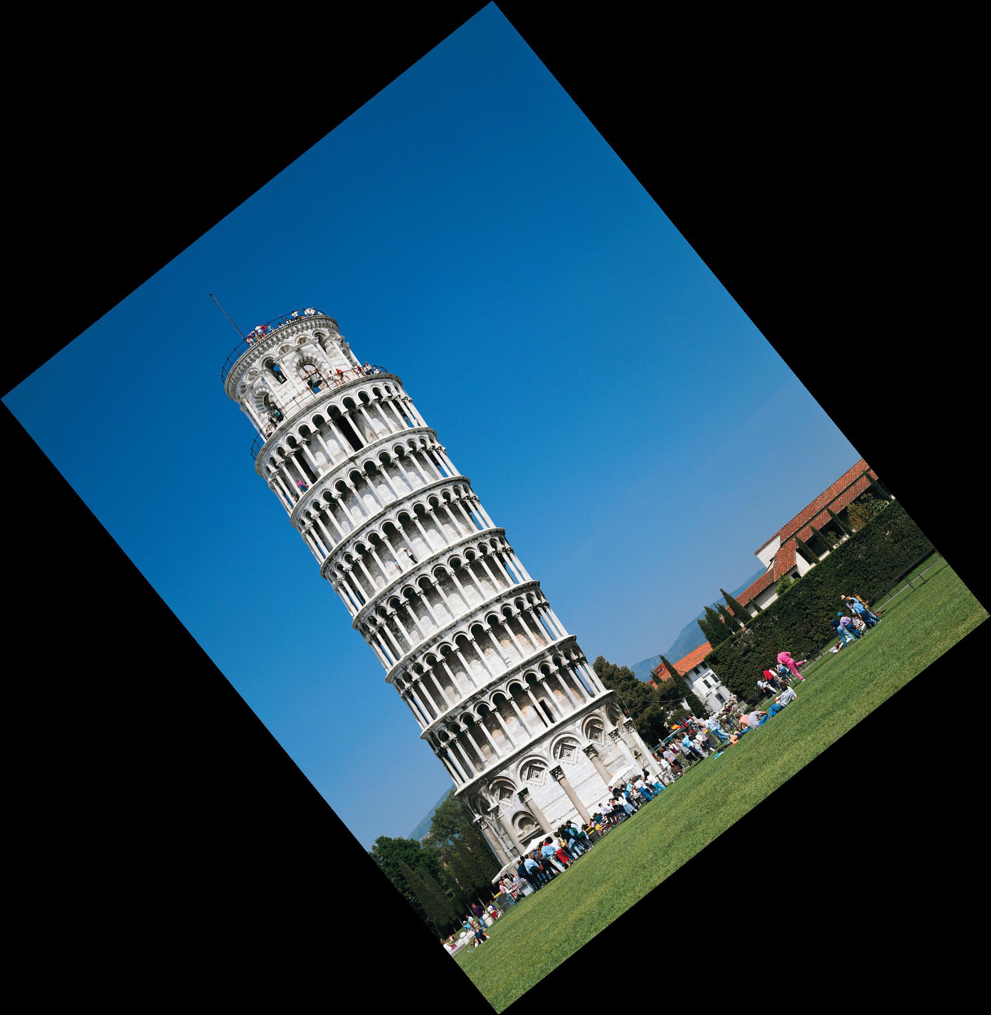
The results for straightening turn out to be pretty good.

2 Fun with Frequencies!

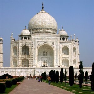
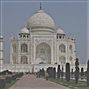
2.1 Image Sharpening

To sharpen an image, we subtract the low frequencies from the original blurry image. Since an image looks sharper if it contains stronger high frequencies, we manually add some high frequenceis to the image by convolving the image with an unsharp mask filter.

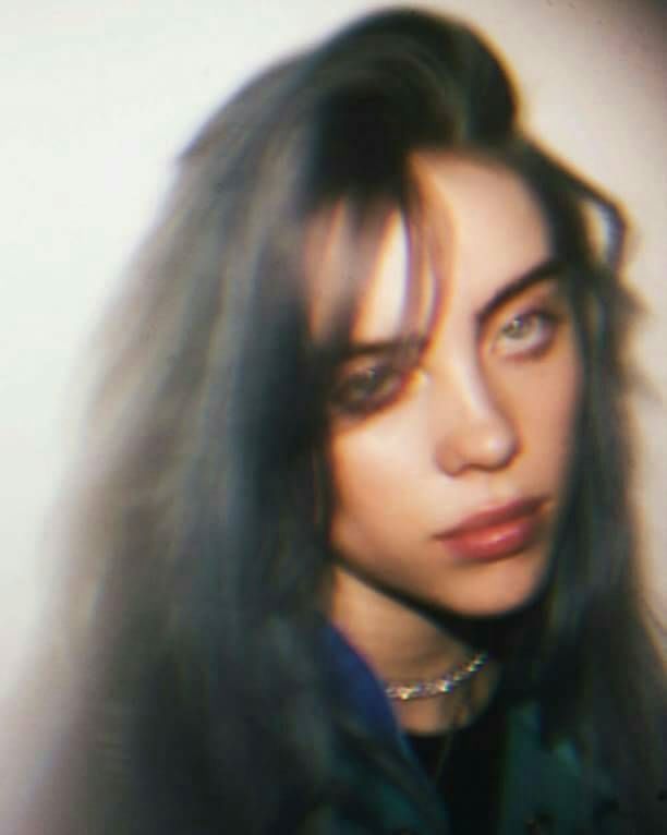
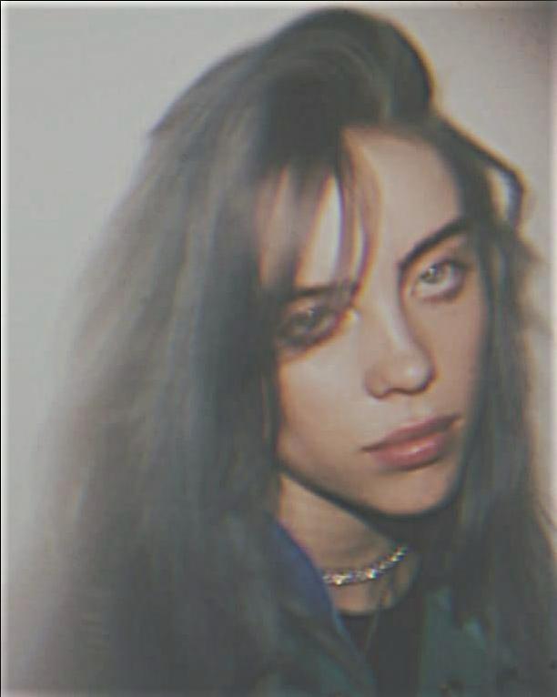
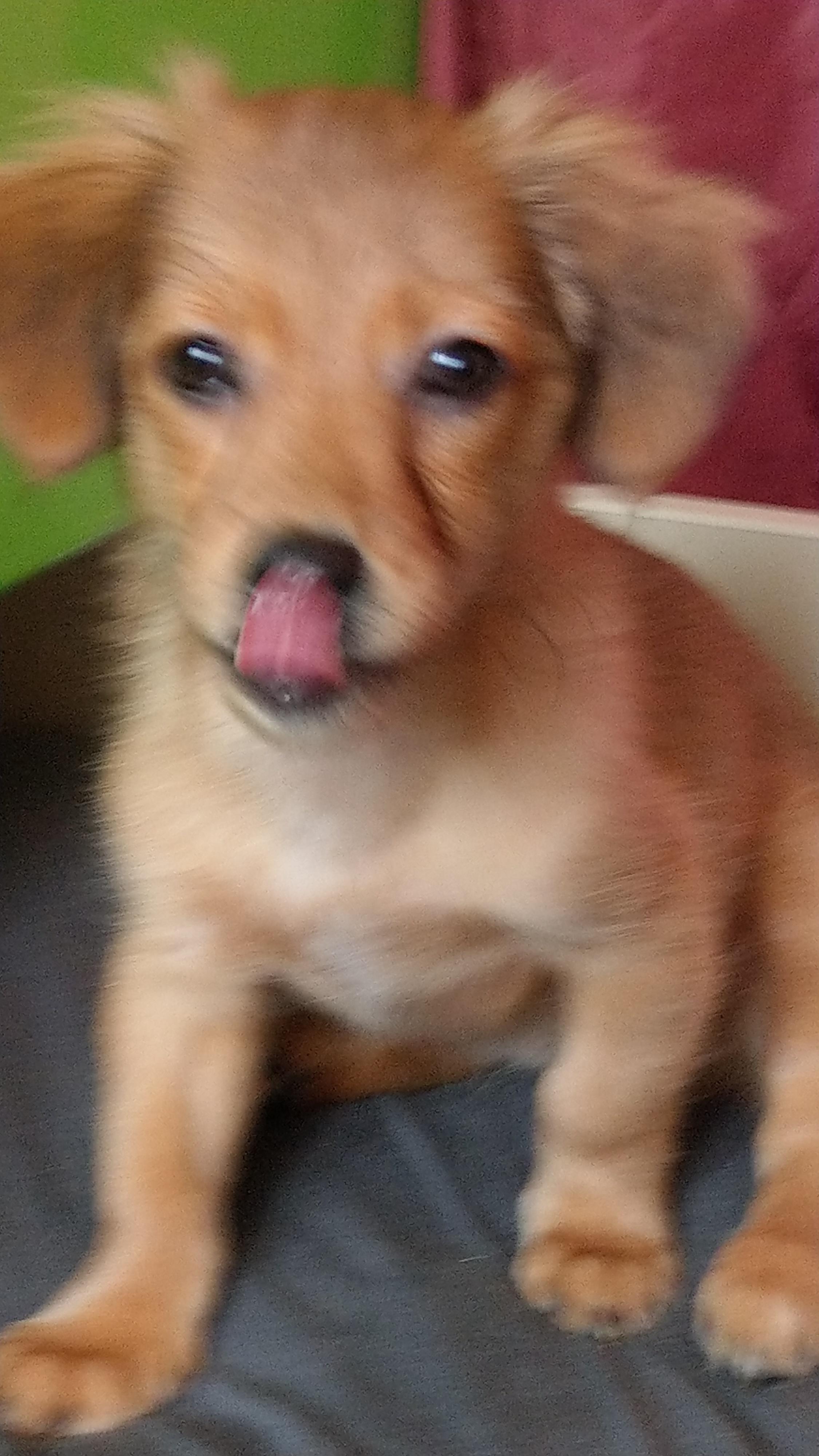
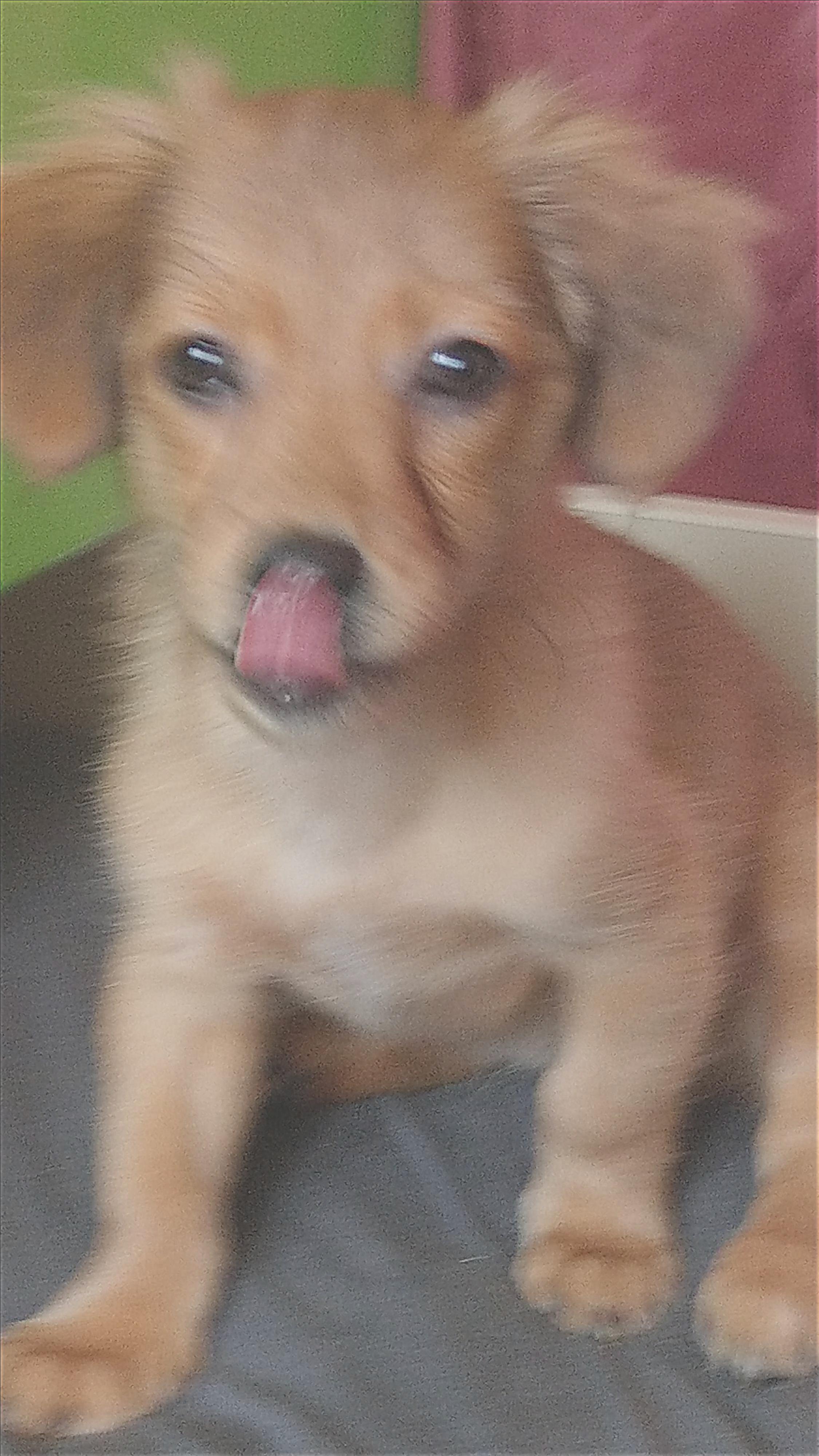
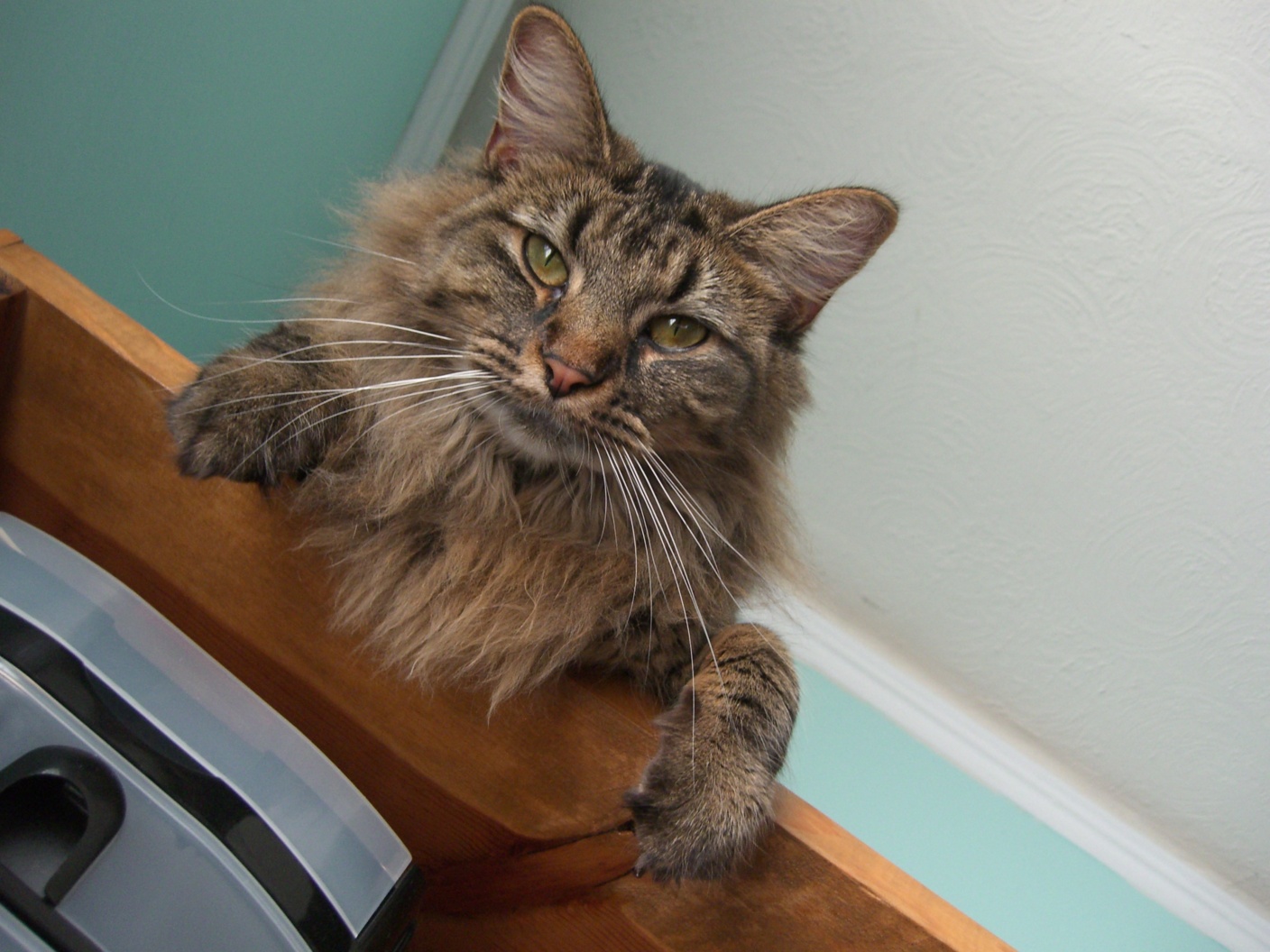
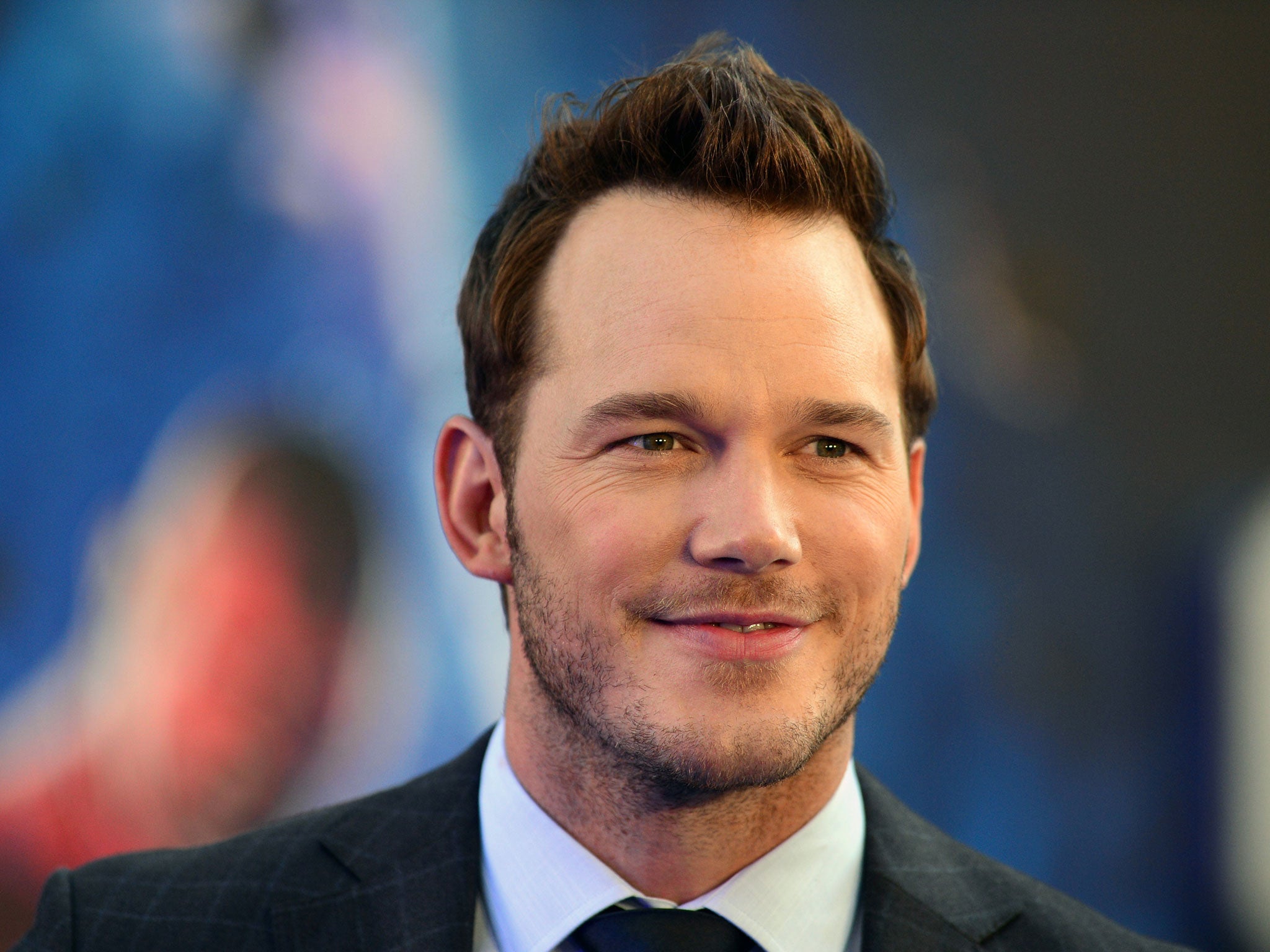
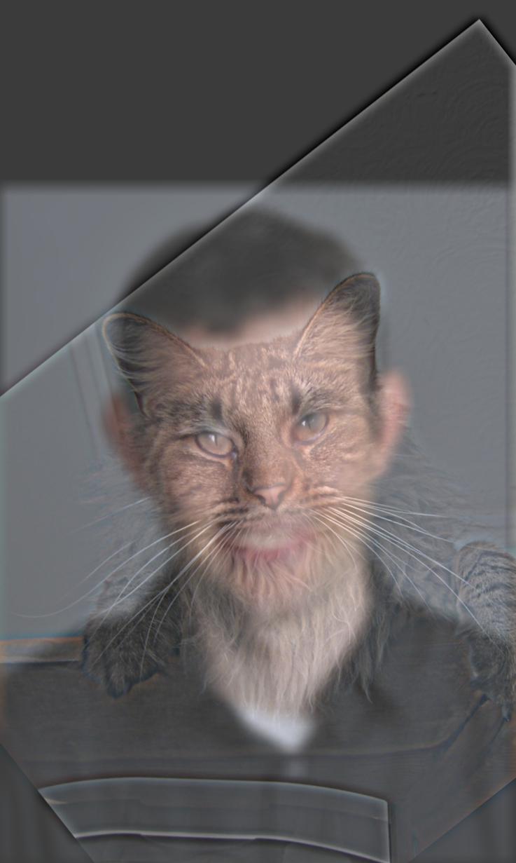
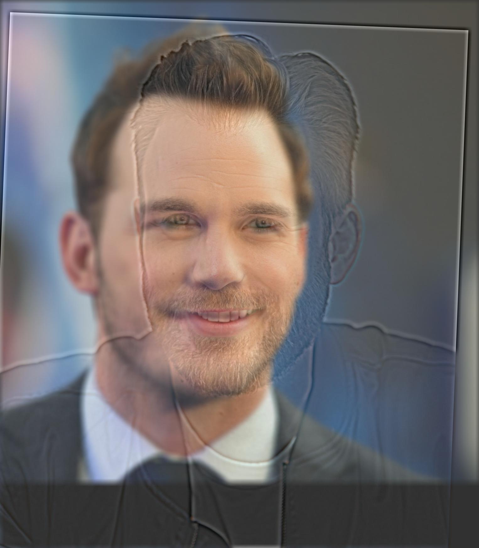
2.2 Hybrid Images

To create the hybrid images, we follow the approach proposed in the SIGGRAPH 2006 paper by Oliva, Torralba, and Schyns. The basic idea is that high frequency tends to dominate perception when it is available, but, at a distance, only the low frequency (smooth) part of the signal can be seen. By blending the high frequency portion of one image with the low-frequency portion of another, we get a hybrid image that leads to different interpretations at different distances.

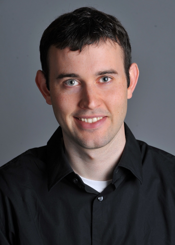
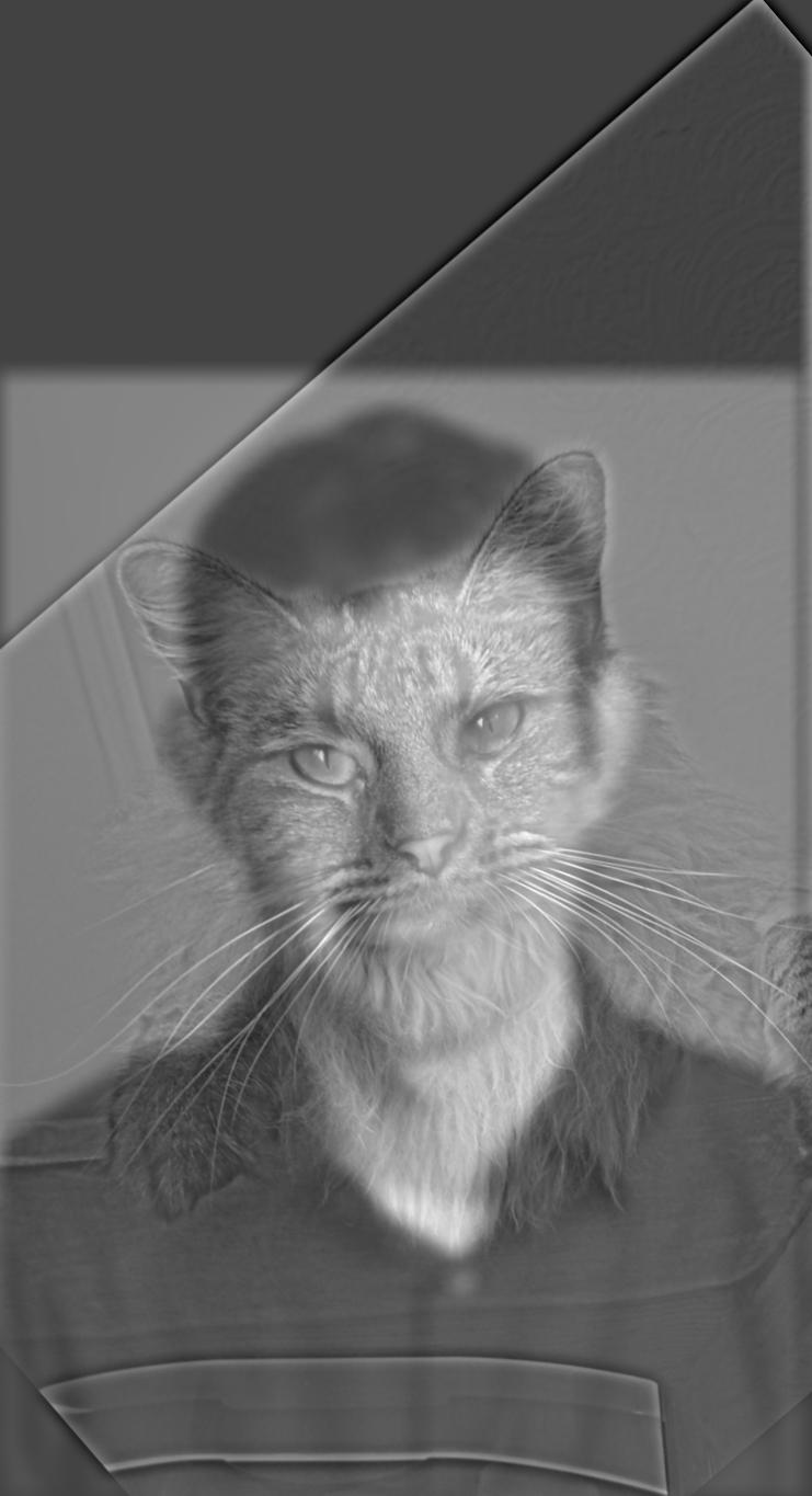
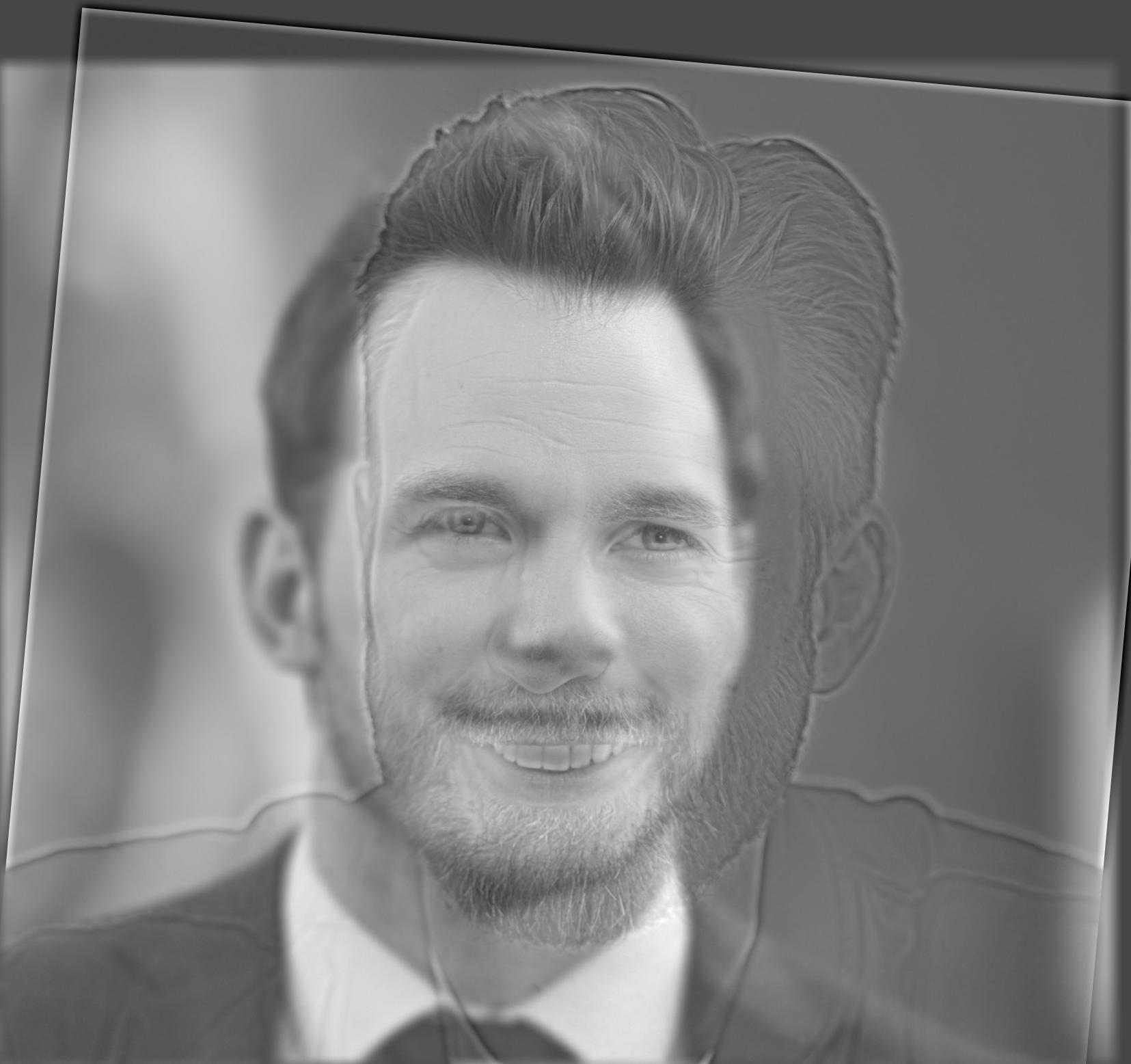
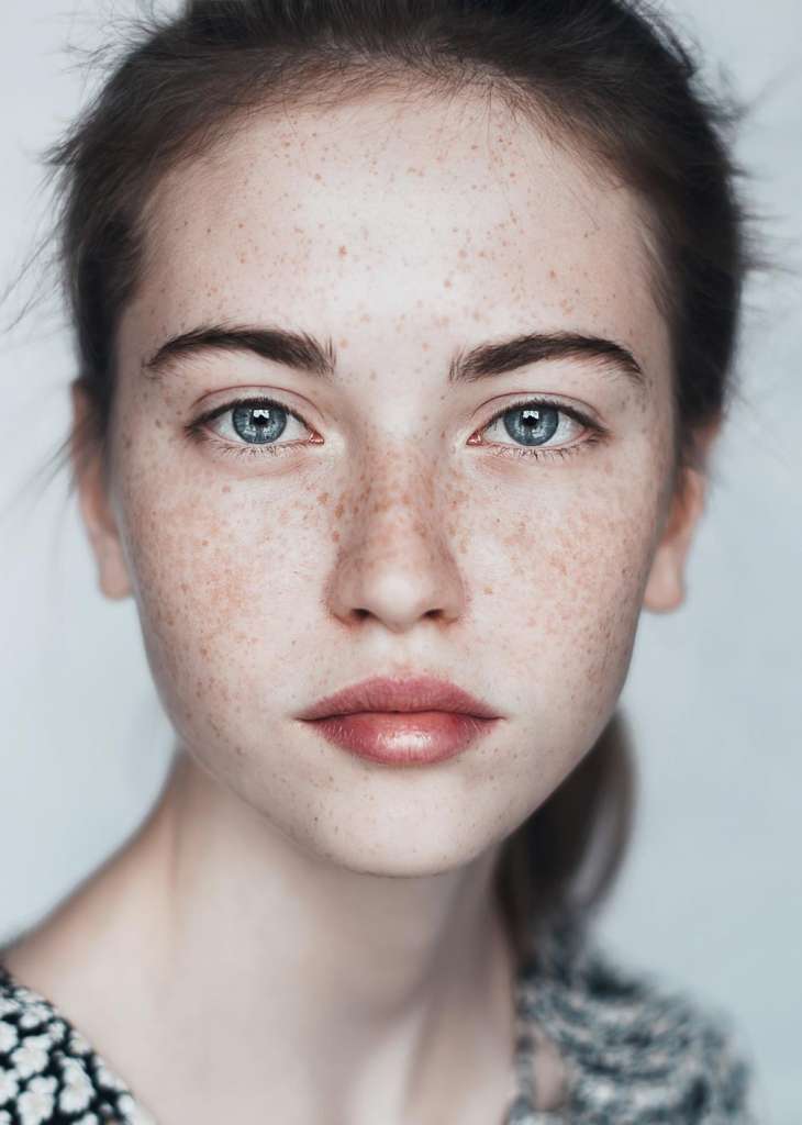
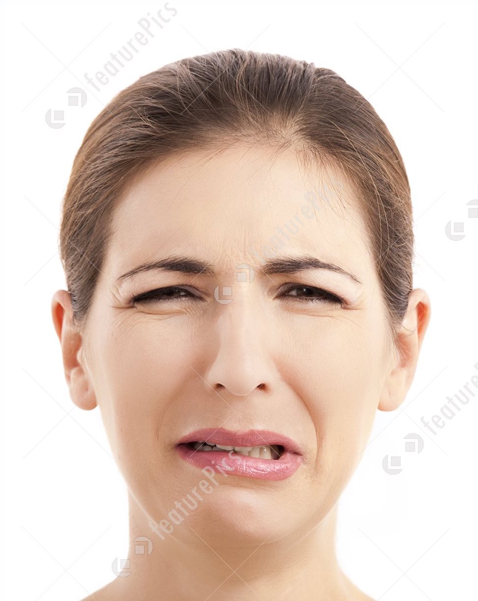
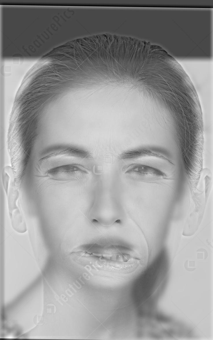
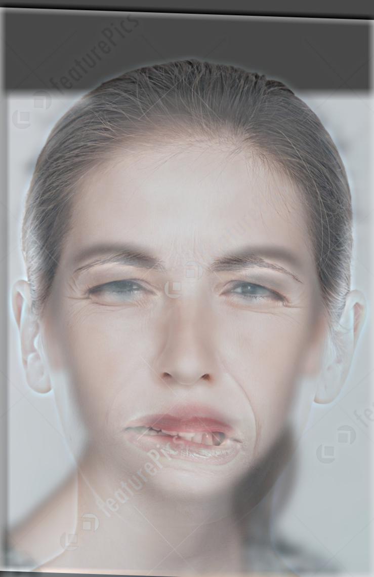
The above image of change of expression is my favorite result. You can see a sad face when looking closely while seeing a peaceful face when looking from far away.

2.2.1 Using Colors!

To use colors, we simply apply the filters to all the color channels! These are the results:

2.2.2 Fourier Space Analysis

My favorite result is the mix of the two facial expressions, both using color:

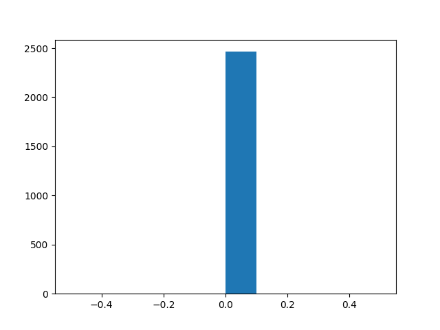
We, now, compute the 2D Fourier transform for booth images:

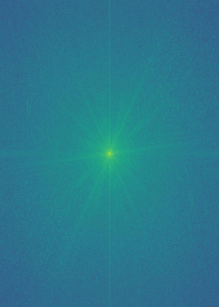
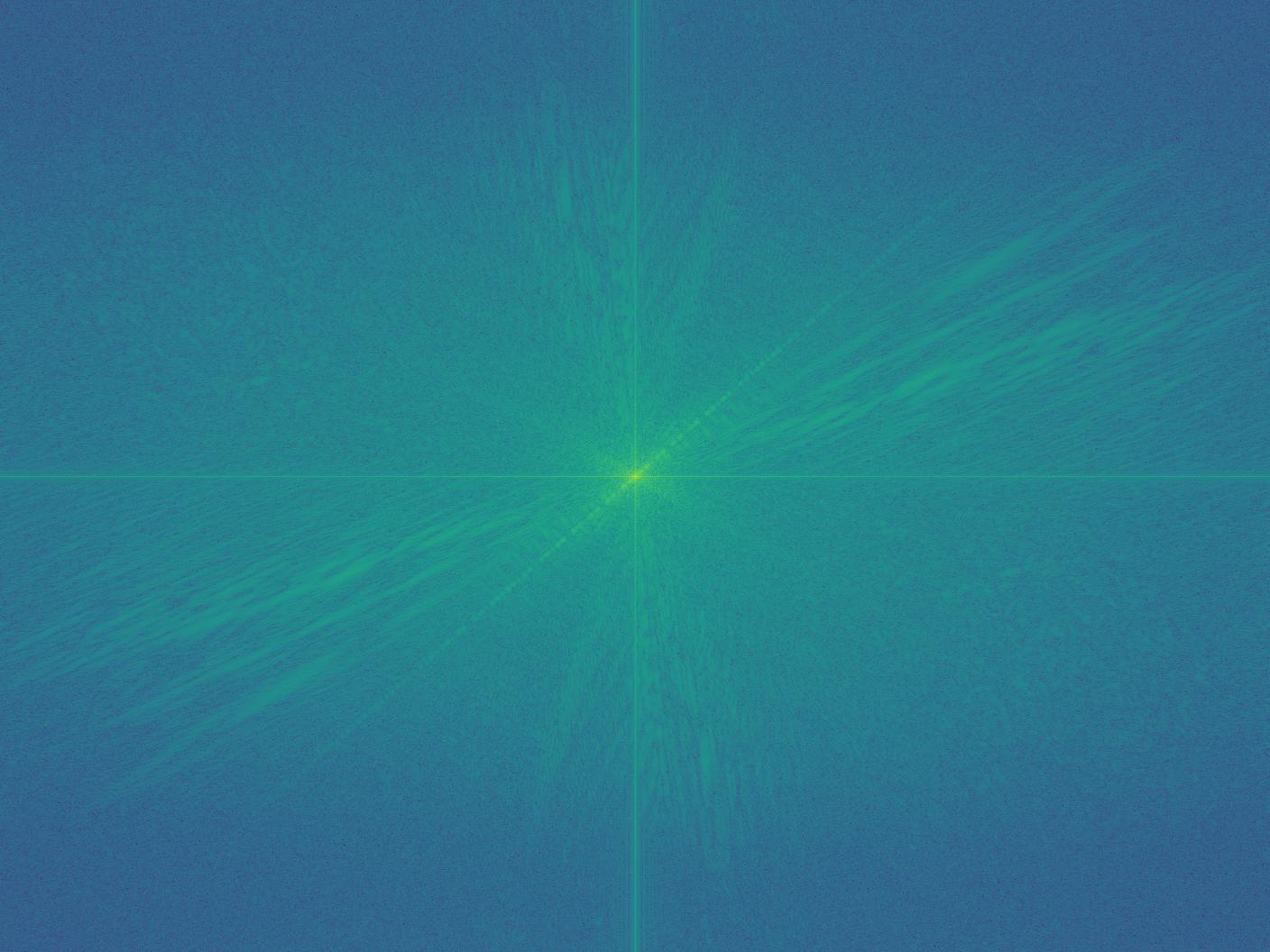
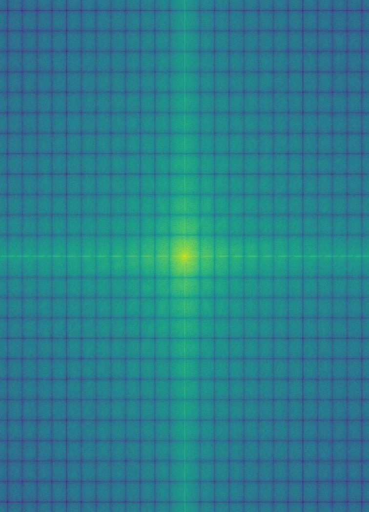
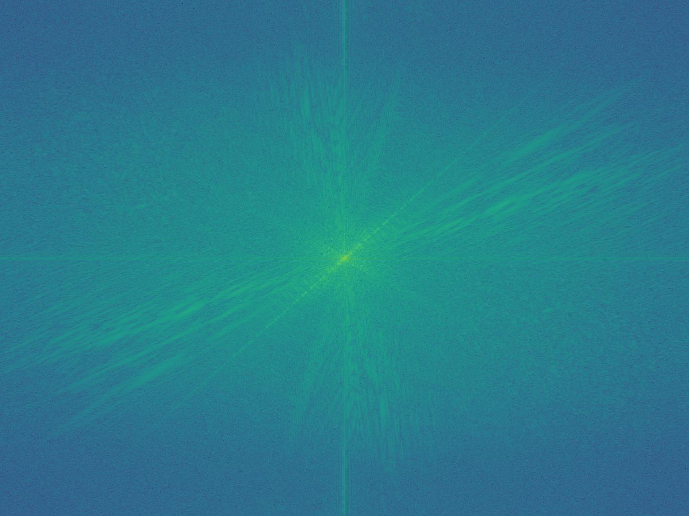
The natural face after Gaussian filter and the sad face after Laplacian on Gaussian filter

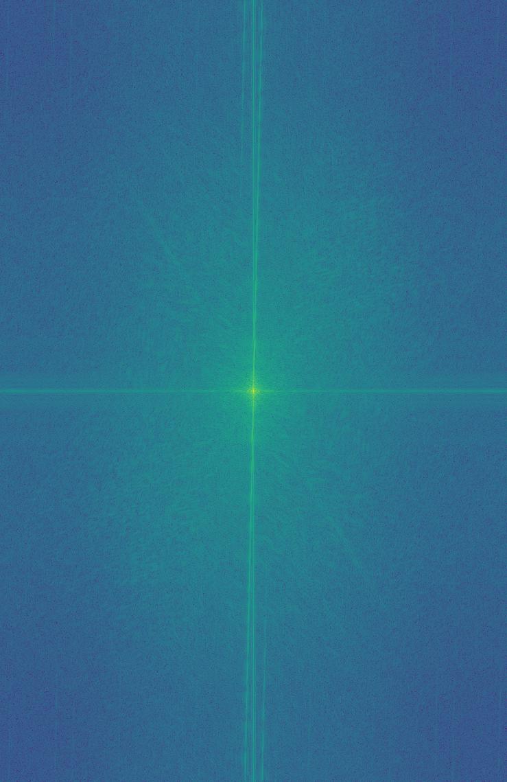
Hybrid image product

We can see, from the Fourier space filtered images and their sum, that, once they are added to each other, the low frequency image has its gaps filled by the other, and the high frequency has its low frequency spectrum intensified by the other.

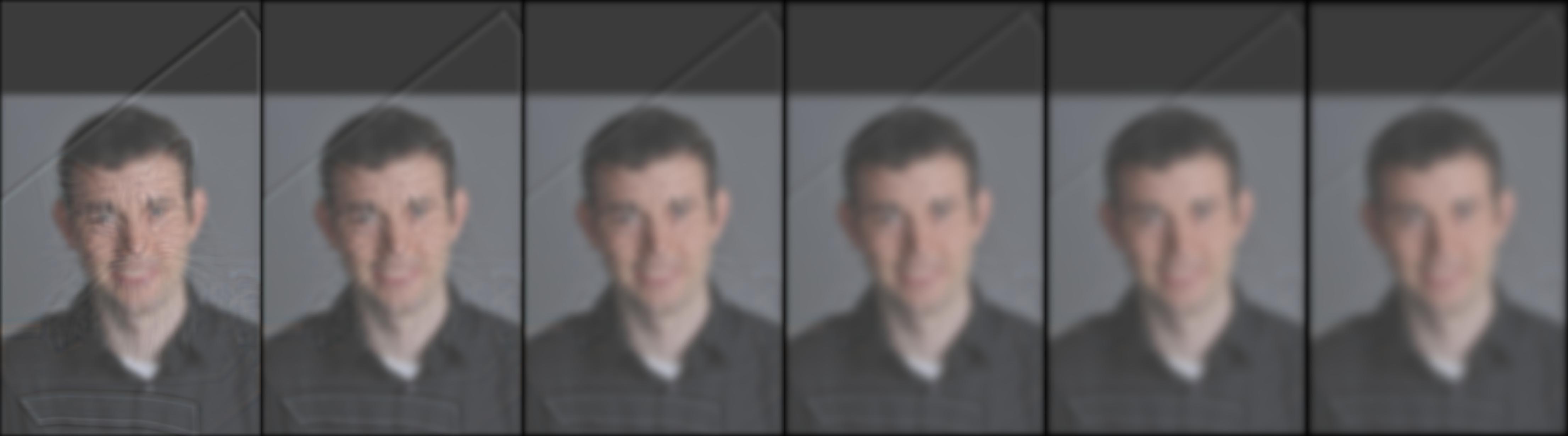
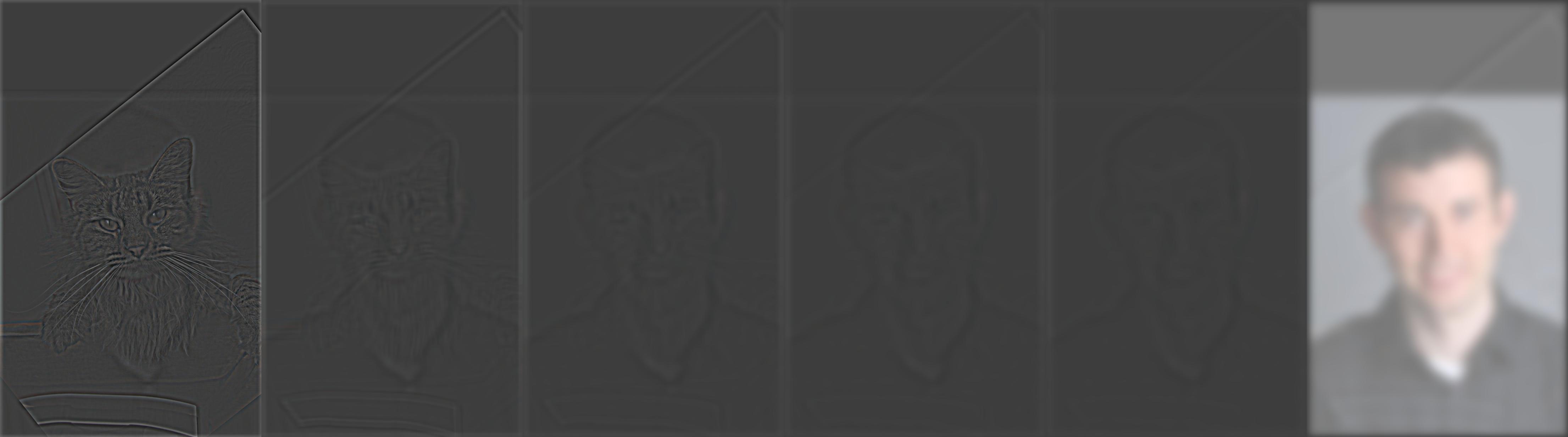
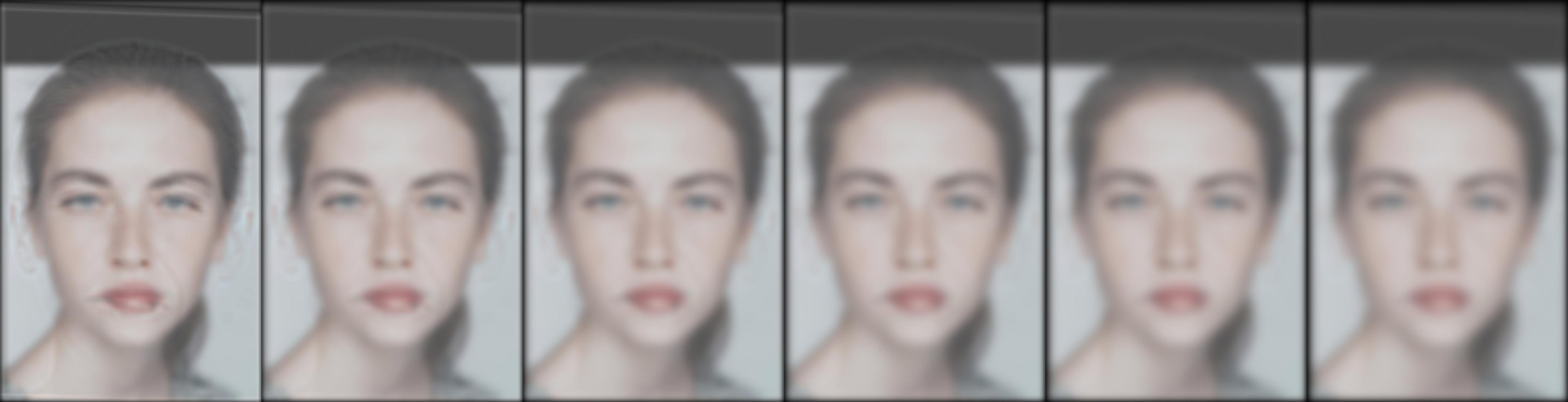
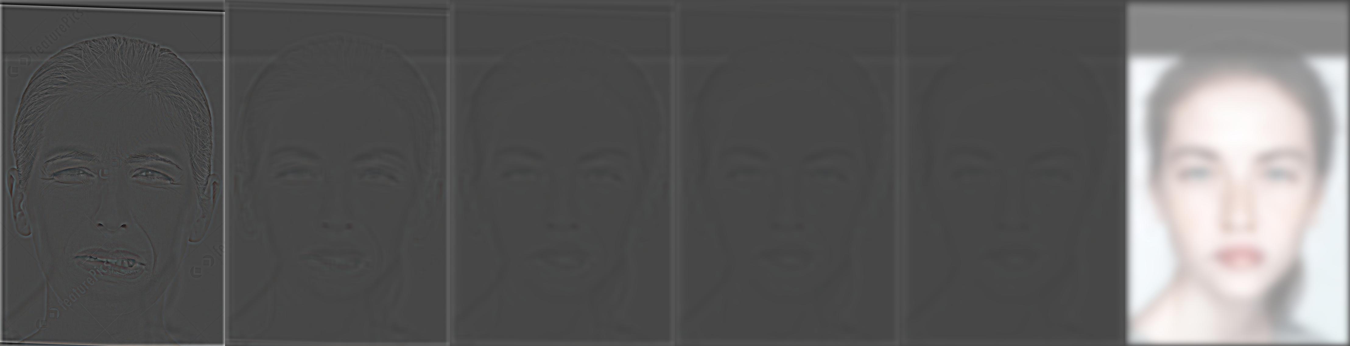
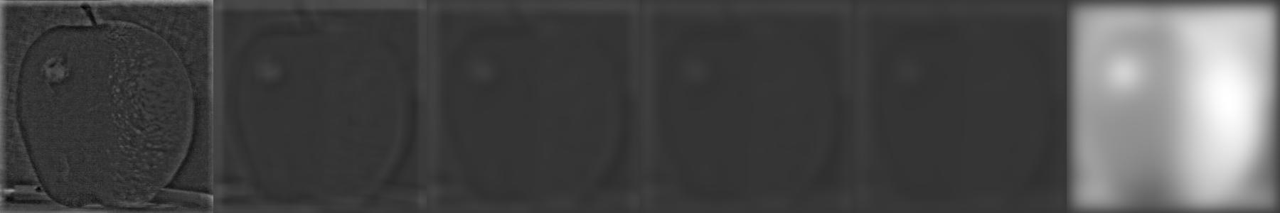
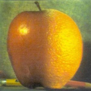
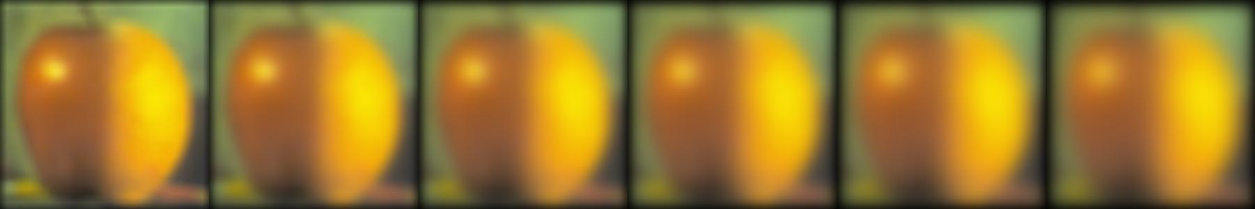
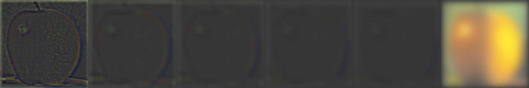
2.3 Gaussian and Laplacian Stacks

We then implement Gaussian and Laplacian stacks to observe the structure at each resolution. To create the successive levels of the Gaussian Stack, just apply the Gaussian filter at each level, but do not subsample. In this way we will get a stack that behaves similarly to a pyramid that was downsampled to half its size at each level.

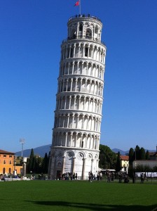
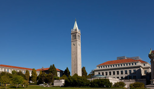
2.4 Multiresolution Blending

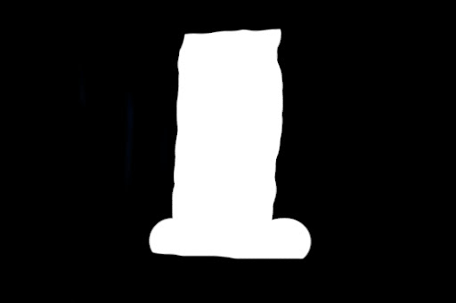
We then blend two images seamlessly using a multi-resolution blending as described in the 1983 paper by Burt and Adelson. An image spline is a smooth seam joining two image together by gently distorting them. Multiresolution blending computes a gentle seam between the two images seperately at each band of image frequencies, resulting in a much smoother seam. I used the following Matlab code to generate binary masks.

img = imread(img_path);
h_im = imshow(img);
circ = drawcircle();
BW = createMask(circ);
imshow(BW)

2.4.1 Using Color!

3 Summary

I enjoyed this project because it provides a lot of insights into image manipulation. I think it's really cool to play with frequencies and change a natural image to something unnatural, such as the photos shown in the Hybrid image section. I would absolutely like to look into this area in the future.