Fun with Filters and Frequencies!
Ja (Thanakul) Wattanawong
Part 1 - Finite Difference Operator, DoG, and straightening
This project was a chance to play with a lot of cool applications of filters and frequency-based transforms of images. For the first part I created a small edge detector based on the magnitude of the gradient of the image.
Computing the gradient starts with the Finite Difference operators  and
and  (for the x and y direction respectively), which we use to approximate the derivative. After convolving each of these with the image we will have gradient in the x and y directions, after which the element wise magnitude can be calculated using
  . Then we can binarize the image based on a cutoff to see the edges.
1.2: Then, we used the derivative of the gaussian filter to improve edge-finding. This made the edges much more prominent in the gradients since the high-frequency signals were removed and we could turn the sensitivity way up without introducing noise.
After that we worked with the angle to straighten images:

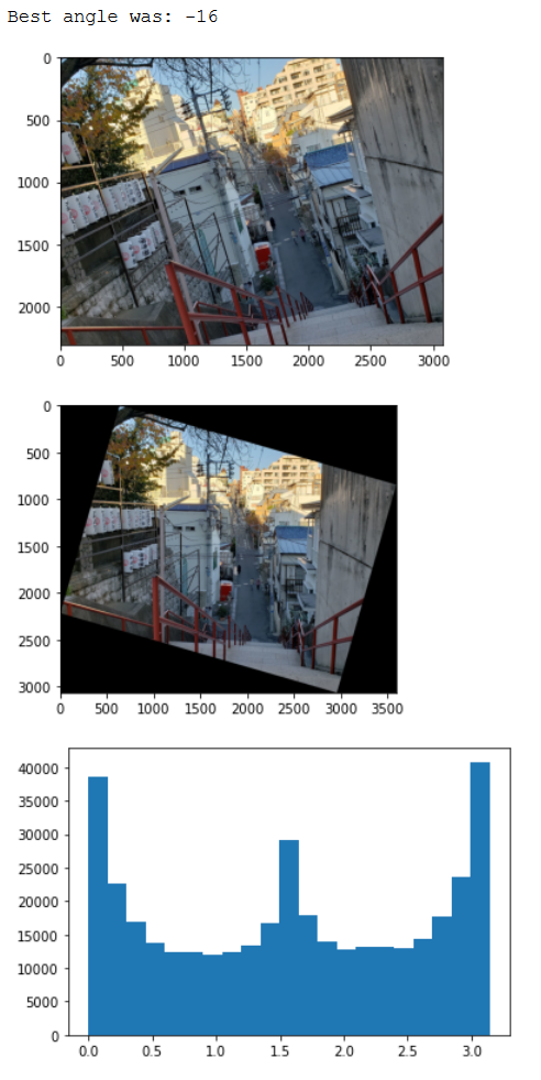
![]()
The failure case here is likely because there were not a whole lot of lines to be detected in the x axis so it considered this to be a fairly good rotation. The rest worked really well however.
Part 2
Part 2.1 - Sharpening
Here we played with the unsharp mask filter which generally improves perceived detail at the cost of noise.
To get a clearer image (lol) of why this is sort of “fake” let’s try an example on a blurred image:


Clearly even with this unsharp mask filter we are unable to regain the high-frequency signals lost in the blurring process, and turning sigma way up will only cause artifacts like ringing.
Part 2.2 - Hybrid Images
Next we played with hybrid images that exploit how we perceive high-frequency elements better when we’re closer to the source and vice versa.


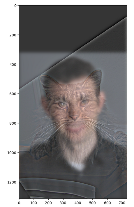
On the right side is a Fourier transform of both source images in grayscale. You can see that Derek’s image corresponds to the one that is focused around the center and axes due to absence of high-frequency elements, while the cat image retains high-frequency elements and attenuates the low frequency ones.
I started with color and it produced good results. Trying both grayscale also produced okay results. Making only the high frequency one colored introduced weird colors in the overall image, but making only the low frequency one colored didn’t change too much from using both colored. In general using both colored seems best though this is dependent on the image pairing.
Here are examples of a few more:


The last one is kind of a contrived example but shows you can’t do this for arbitrary images. It’s difficult to distinguish earth once it’s blurred, especially when the sun has such intricate patterns that dominate even when you look from far away. The end result is a somewhat amorphous and mystical ball.
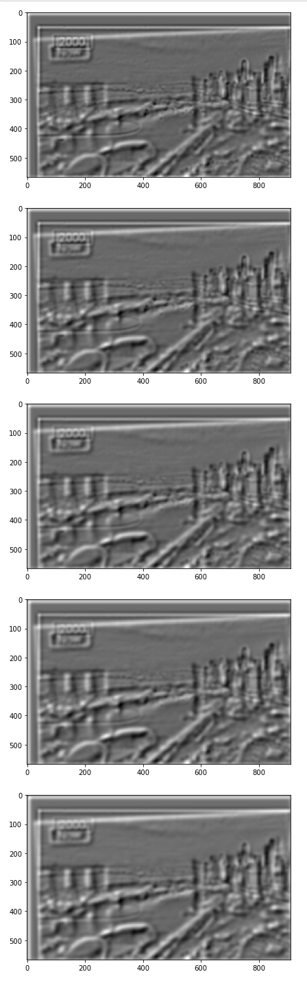
Part 2.3 - Gaussian and Laplacian Stacks
I picked the hybrid image of Singapore to show the different elements and show where different frequencies show up in each stage.
Part 2.4 - Multiresolution blending
The Oraple in color!:


Before and after:


Now we know who really built the Stonehenge (I admit the UFO doesn’t really count)...


Conclusions
This was really fun! I got to learn a lot about the mathematics behind a lot of things that Photoshop does and play with a lot of cool images.