CS194-26 Project 2

Kevin Shi

Overview

This project consists of multiple parts, and is an exploration of multiple filters and their applications to image sharpening, blending, rotation, and human vision.

Part 1: Fun with Filters

Part 1.1: Finite Difference Operator

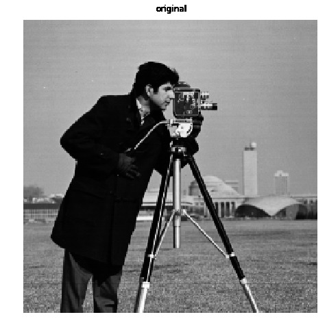
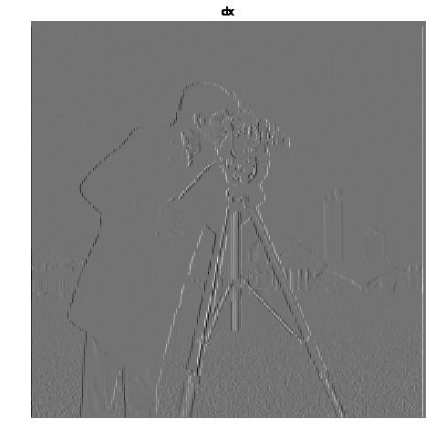
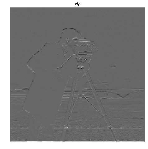
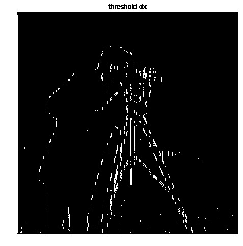
Here we work with finite difference operators dx and dy to find the edges of the image.

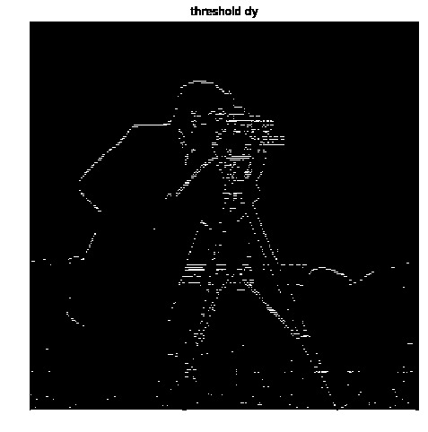
We have a lot of noise in this image and it is very difficult to remove. Removing the noise also removes a lot of the actual edges. I went through multiple thresholds to find a good compromise between edges and noise, eventually landing on 0.21

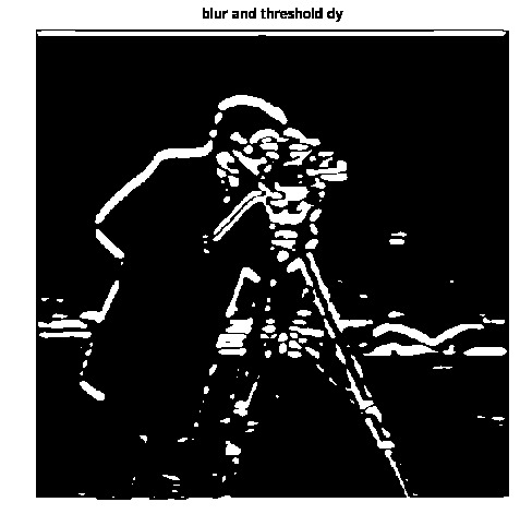
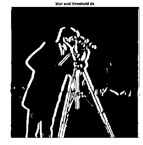
Part 1.2: Derivative of Gaussian (DoG) Filter

Here we work with guassian filter to blur the image to get rid of noise. Then afterwards derive to get cleaner edges.

In this below example we guassian blur first with a kernel size of 20 and a sigma value of 3. As you can see, this removes a lot of the noise so that we can have a lower threshold value of 0.018. We can also see that this makes the lines fatter, which happens because we are also blurring the edges, making them thicker.

We then convolve the gaussian kernel and the finite difference kernel first before then convolving with the image. This yields no difference between the outputs because convolution is associative. This however should run faster because the convolution between the smaller kernels is done first.

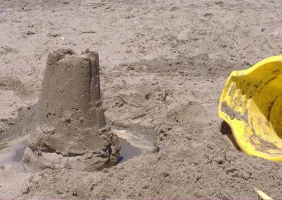
Part 1.3: Image Straightening

Here we attempt to rotate an image to be straight and upright automatically. We do this through the assumption that most of the edges in an image are vertical and horizontal.

This algorithm is one that straightens images based on the assumption that most lines will be horizontal and vertical. My algorithm detects these lines through a couple of steps

It blurs and derives the image.
Calculates edge strength and gradient direction. Gradient direction is given only by angles in the first quadrant for simplicity of calculation
Finds lines by thresholding the gradient direction matrix by the edge matrix
Calculates a histogram of the angles
Proposes rotation angle based on the median of the histogram group with the most angles
Tries both clockwise and counter-clockwise rotation (+/-) - this is due to the simplification in step 2 of angles only being in the first quadrant.
Calculates vertical and edge lines to find the right rotation

The gradient magnitude computation is done by finding the l2 norm of [fdx, fdy]. The gradient angle is given by arctan (dfdy / dfdx).

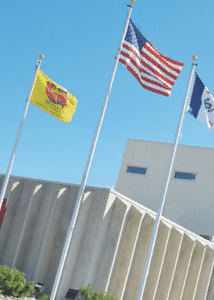
Let us run through a example so we understand the process

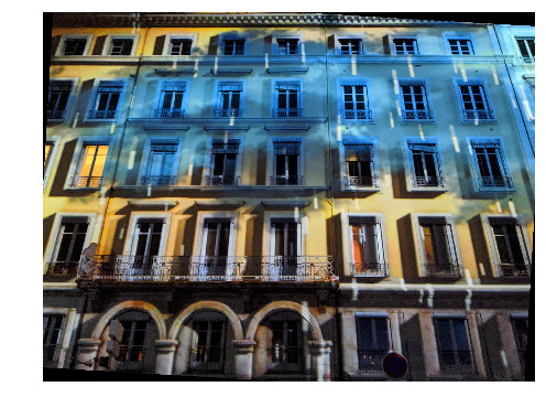
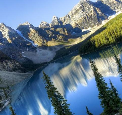
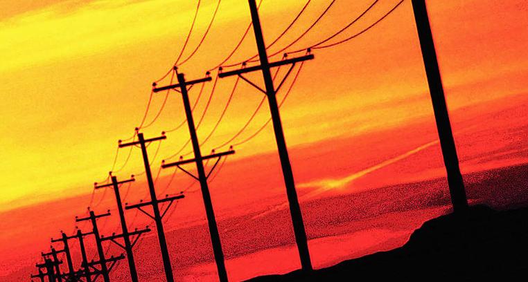
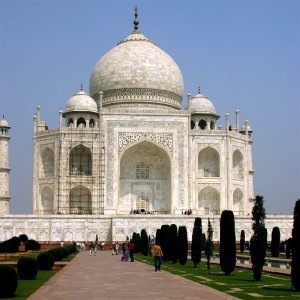
First we have the original image:

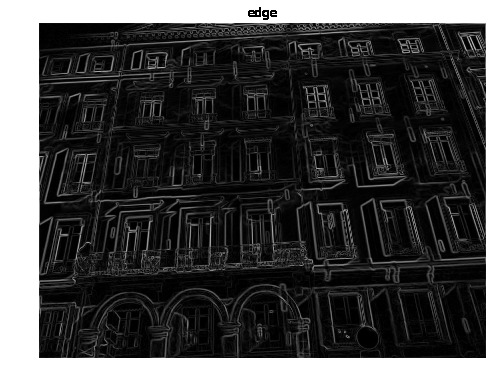
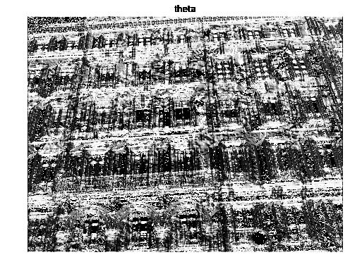
Next we derive and blend like in 1.2 except without binarize thresholding(1). Using this, we calculate the gradient angle and edge matricies (2):

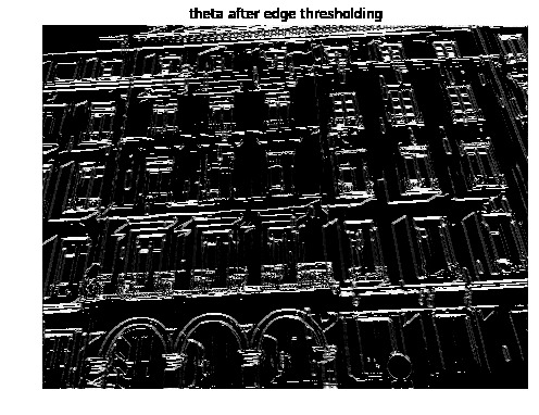
Then we find the angles we care about, which are the ones on the edges (3):

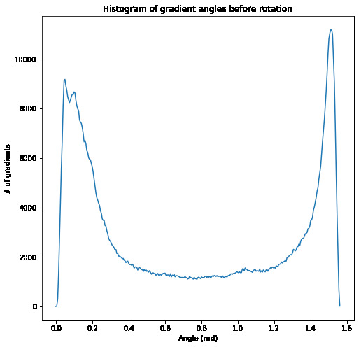
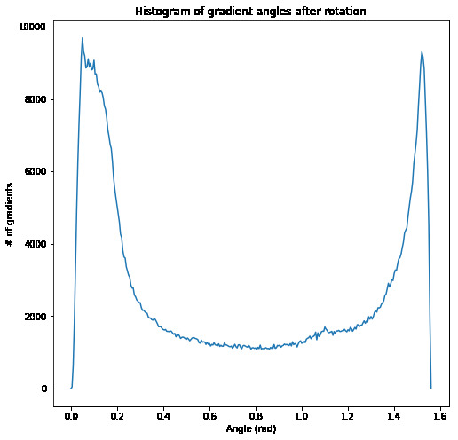
Then we calculate the best rotation by looking at the histogram(4)(5):

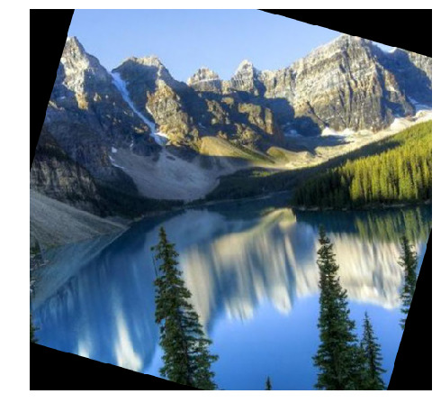
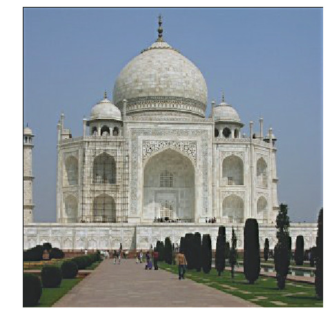
Then we end up with a final rotated image and its histogram

The results here will show our image before and after so that as a human, we can judge how well the algorithm works. Along with the images we will show the histogram of edge angles so that we can see how well the algorithm is actually performing on our assumption.

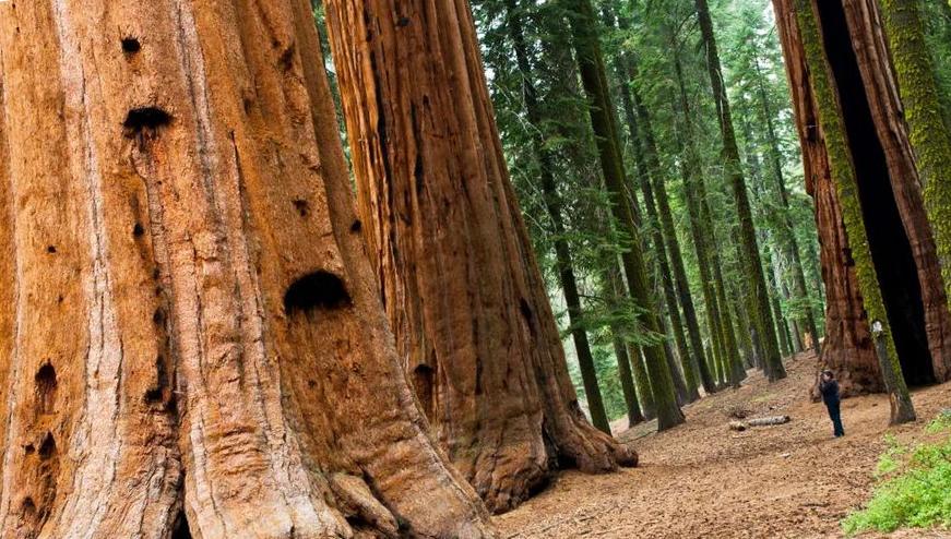
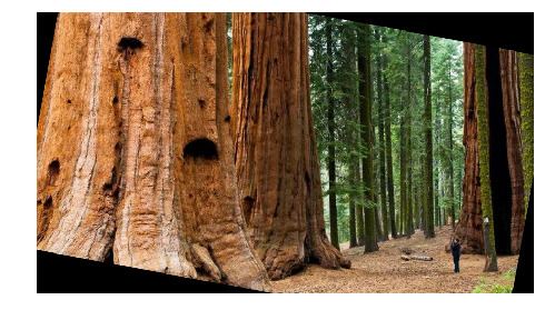
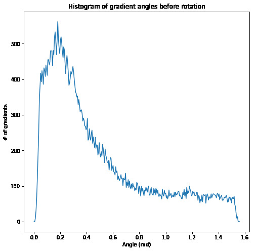
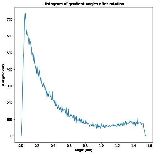
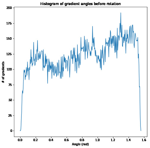
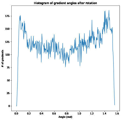
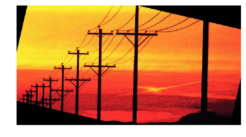
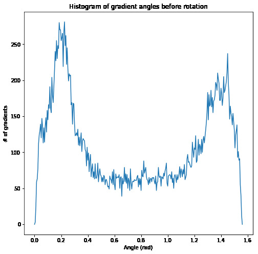
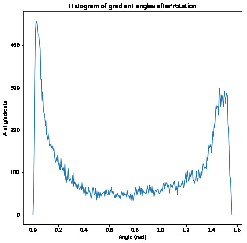
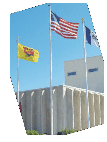
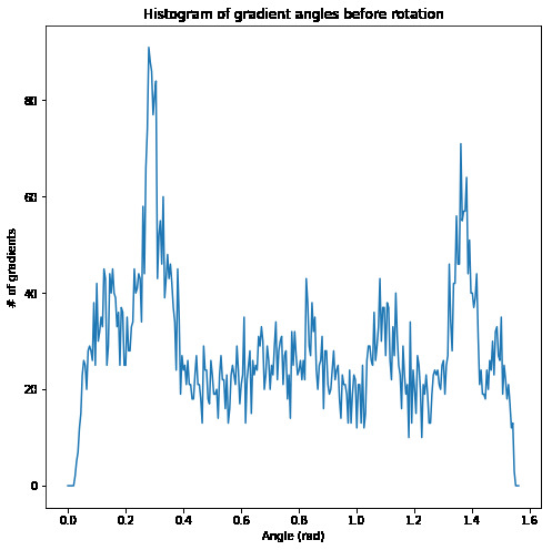
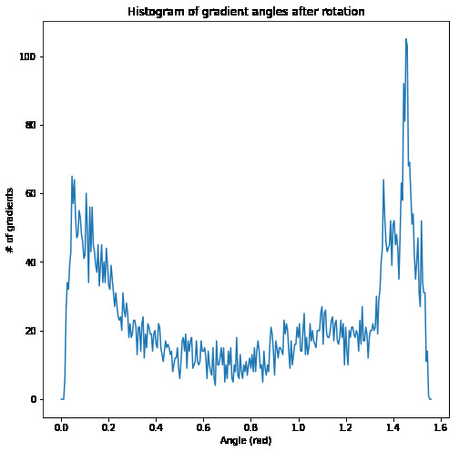
We can see that a lot of the images, especially the images of human made objects, work well with the algorithm. From the histograms, we can see that as we rotate the image, there are more gradients aligned with the 0 rad and pi/2 rad. We can see that these images turn out well, meaning that our assumption was correct.

However, the mountain with lakes image did not rotate correctly. As we can see, the histogram does indicate that our algorithm worked properly as designed and increased the number of horizontal and vertical gradients; however, this does not lead to a visually upright image. This is because our assumption is wrong in this image, and there are often not perfectly vertical or horizontal edges in natural scenes.

Part 2: Fun with Frequencies

Part 2.1: Image "Sharpening"

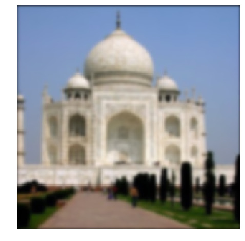
In this picture, I used unsharp filter given by ((1+alpha)*e - alpha*g)- e being the unit inpulse and g being the guassian filter. Then the sharpening is all done in one convolution. Each channel is sharpened, then stacked back onto each other for the rgb image.

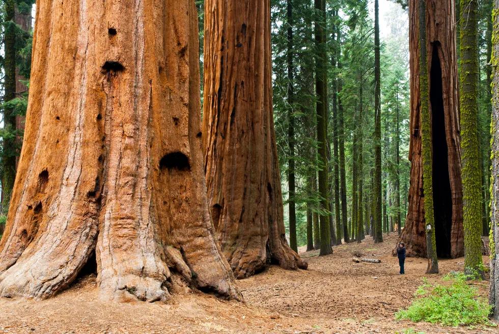
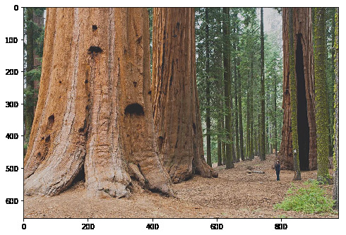
Honestly I don't notice too big of an effect on sharpness. It seems to me the intricate design on the top of the doorway is a little bit more intricate.

Here we will try blurring then sharpening

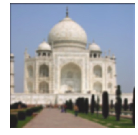
Blurring then sharpening does not seem to have much effect. This is because our unsharp convolution only accentuates the existing high frequencies, but in our blurred image, we do not have high frequency signals.

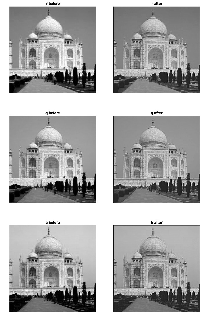
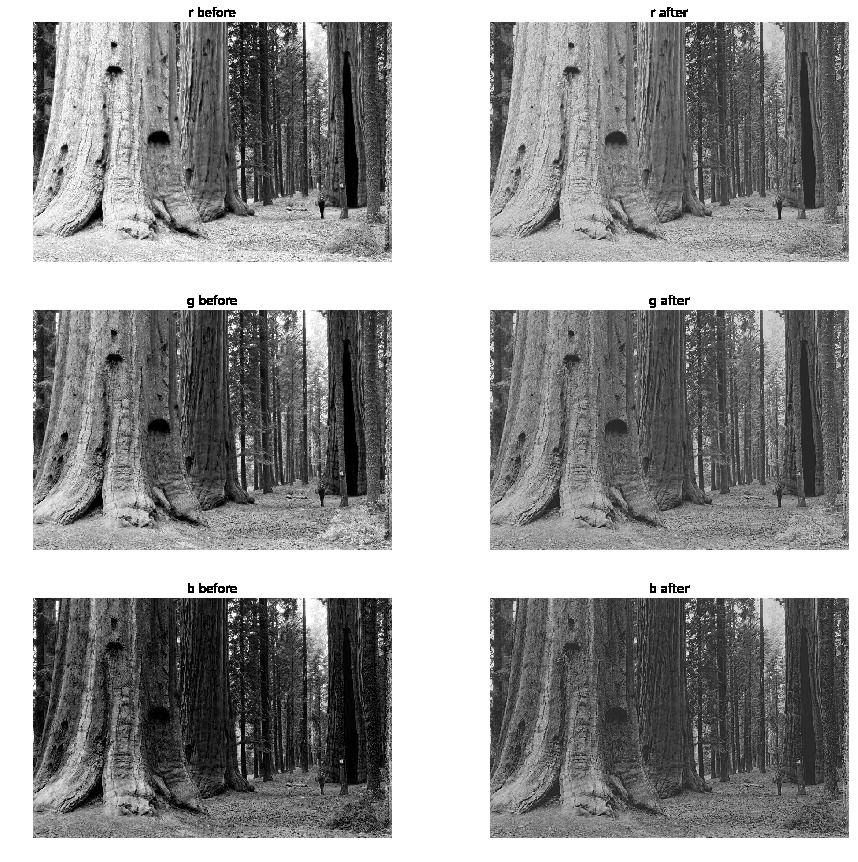
For some reason, sharpening the image using the unsharp filter makes the colors duller. I first thought that this was due to the colors being unbalanced, so I balanced the maximum value of each channel to be the same in the original and new image. However, this did not fix it, leading me to believe that the bright colors are low frequency signals, such as the blue sky or yellow sunlight, that are being masked over by the high frequency signals. However, looking at the before and after of each channel, we can see that the contrast of each channel has been reduced, but I am unsure on how to fix this besides increasing contrast again.

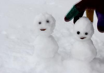
Part 2.2: Hybrid Images

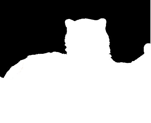
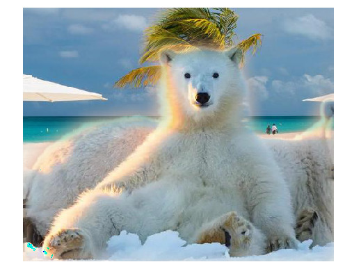
This algorithm aligns the images and then takes the high frequency signals of one image and low frequency signals of another and blends them to make a hybrid image. This was done specifically with a kernel size of 25 a weighted sum of .6 and .4 of the low and high signals respectively.

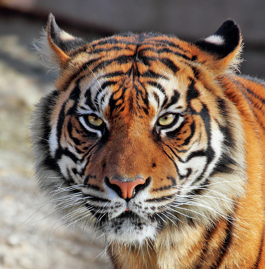
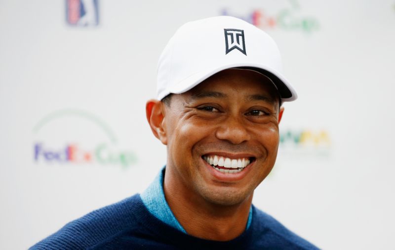
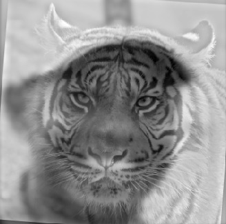
This blended image of Tiger Woods and a Tiger uses sigma values 5 and 8

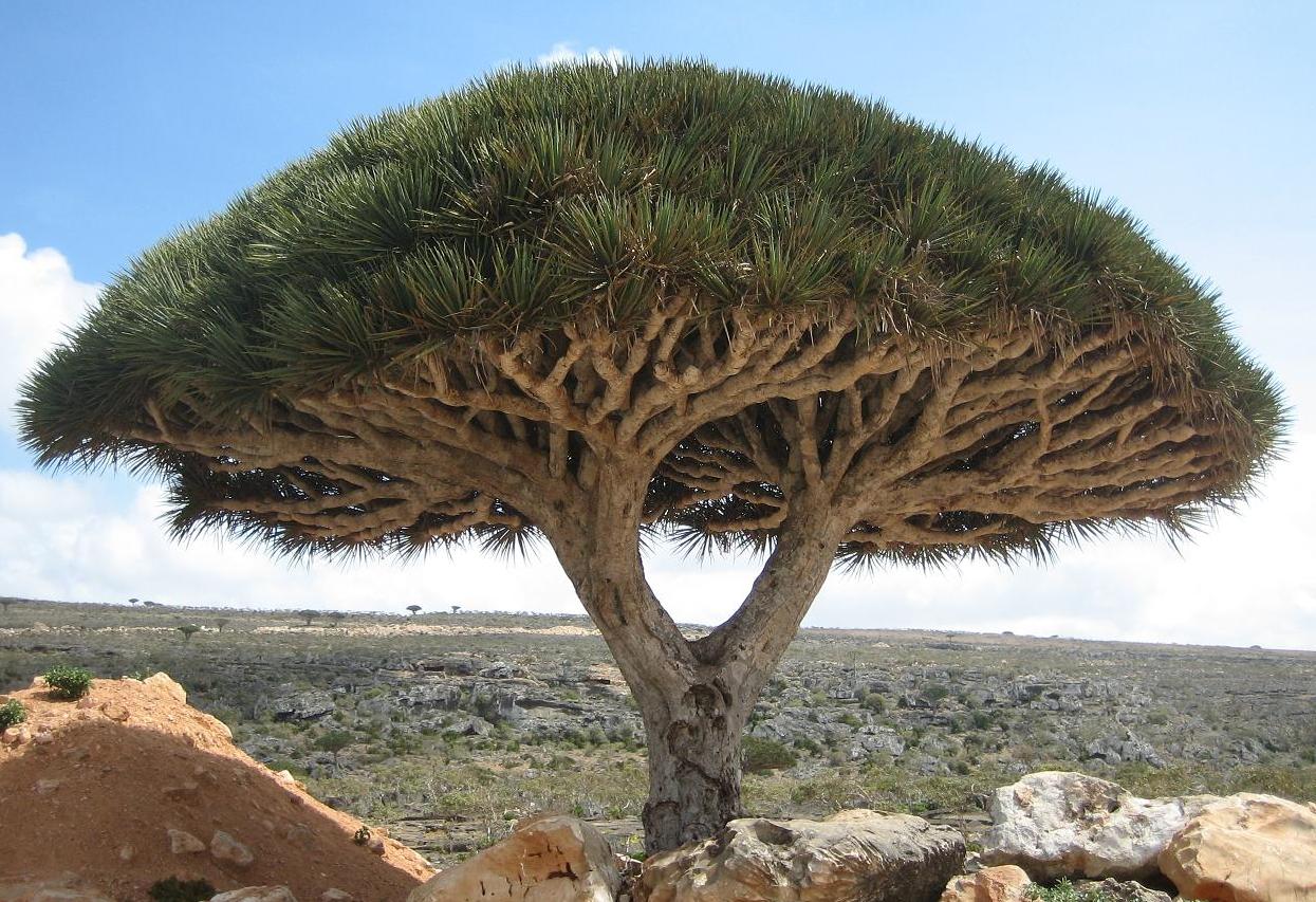
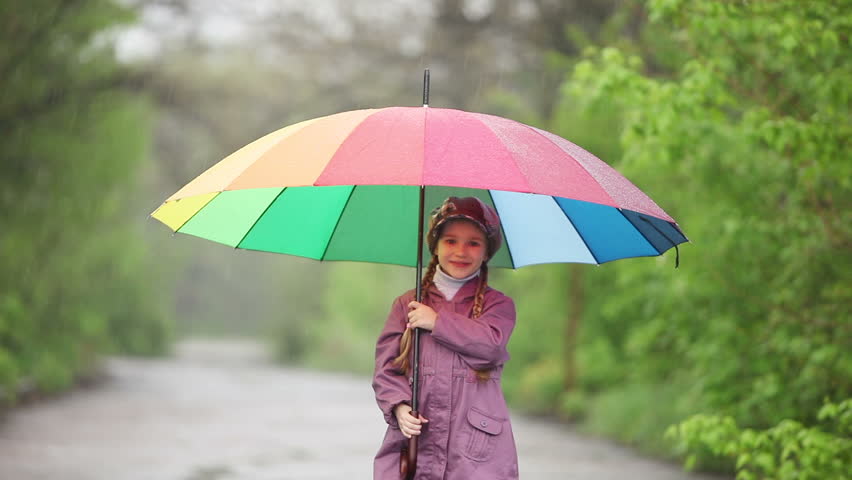
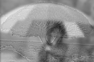
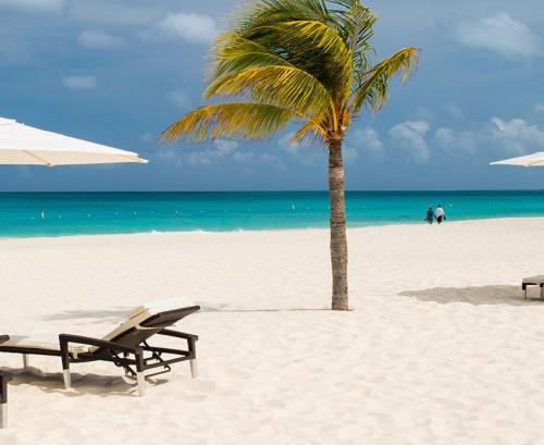
This blended imag of umbrella and the tree uses sigma values 5 and 3

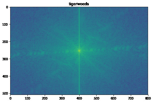
Here we analyze the process of tiger x Tiger Woods through fourier analysis

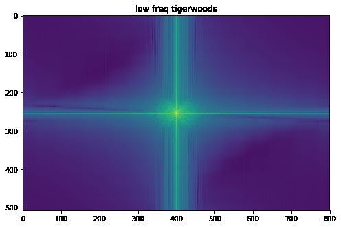
Tiger Woods's fourier transform and filtered low frequency version

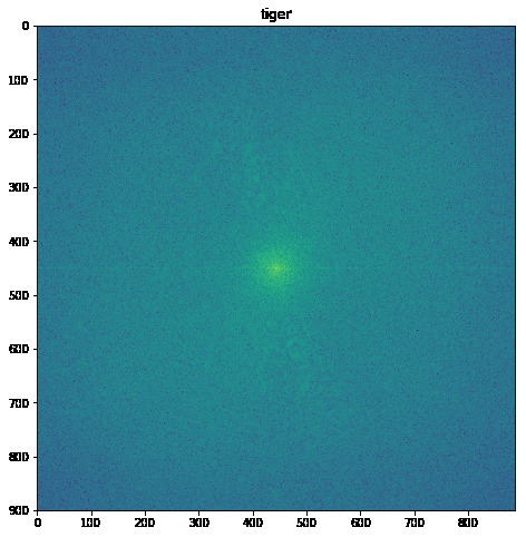
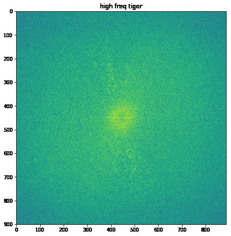
Tiger's fourier transform and filtered high frequency version

Addition of the filtered low and high frequency fourier transforms

We can see in the fourier analysis images that the blended image does look like an addition of the low and high frequency images of Tiger Woods and the tiger respectively.

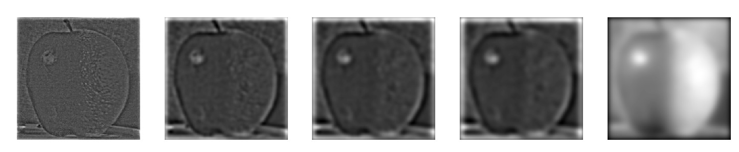
Part 2.3: Gaussian and Laplacian Stacks

Here we make guassian and laplacian stacks. To make the guassian stack, the algorithm just gaussian blurs each layer of the image more and more. To make the laplacian stack, we take each gaussian layer and subtract it from the next layer, getting a specific frequency band.

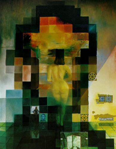
Here we can see the guassian and laplacian stacks of Salvador Dali's painting of Lincoln and Gala

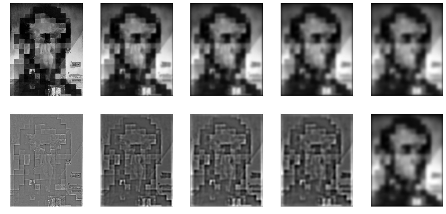
We also look at our previous hybrid picture of tiger x Tiger Woods to analyze it

We can see in clear division of the two images in the laplacian stack

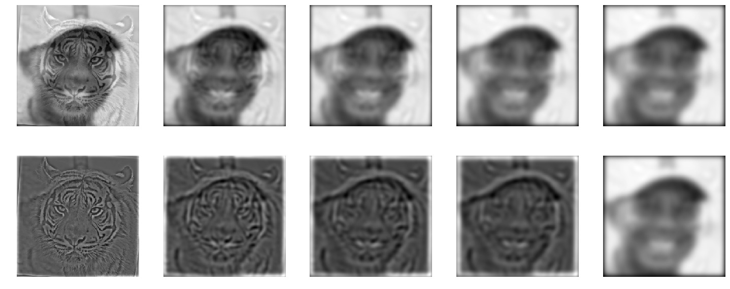
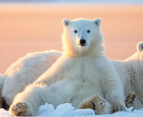
Part 2.4: Multiresolution Blending (a.k.a. the oraple!)

This blending is done through progressively blending each layer of the laplacian pyramid with a higher alpha (aka more aggresively)

Here is the classic example of the oraple:

We can see how its done through our laplacian pyramid

Here are some more examples.

The coolest thing in this project to me was the image straightening using image angles.