Part 1

1.1 Finite Difference Operator

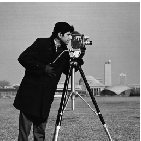
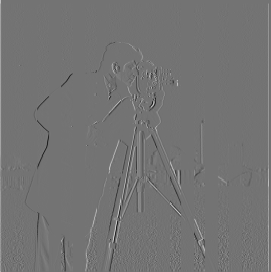
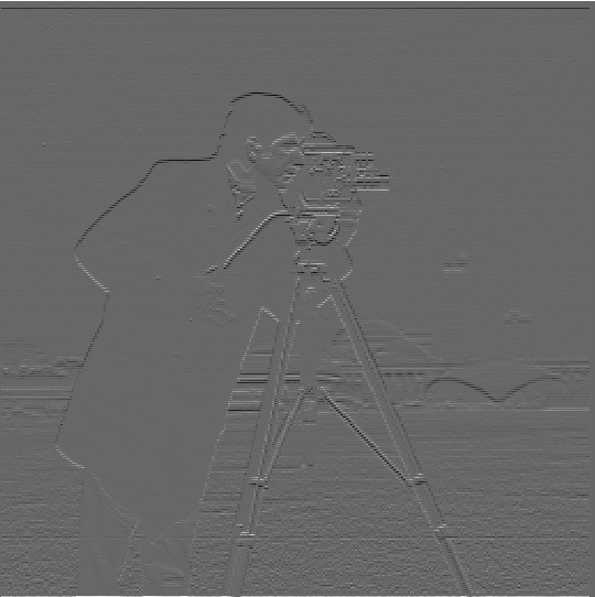
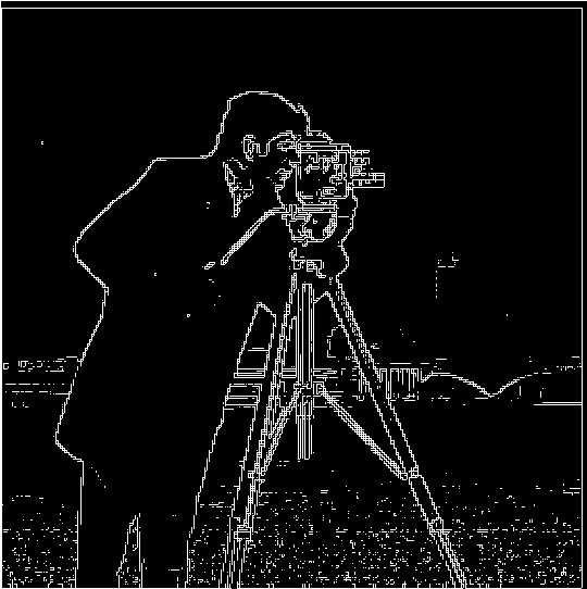
For the gradient magnitude computation, I first convolved the image with [[1, -1]], then I convolved the image with [[1], [-1]]. When I did so, I got the second and third image shown below. After this, for each point in the convolved images, I summed their squares and took the square root, then binarized them, using a threshold of 0.15, to get the fourth image.

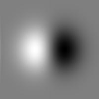
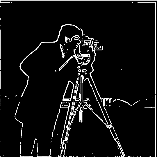
1.2 Derivative of Gaussian Filter

For this part, I blurred the image using a gaussian filter with kernel size 9 and sigma 1. Then, I performed the same calculation I did in 1.1 to get the fourth image below, except with a binarization threshold of 0.09. The image was significantly less noisy and captured the edges more cleanly. However, some details, such as the taller tower in the background, no longer showed up in the blurred image. When performing the convolution between the gaussian filter and [[1, -1]] and [[1], [-1]], I got the second and third images, respectively (though I increased the kernel size and sigma for the sake of visualization). This changed the number of convolutions with the image to two rather than three, and it yielded exactly the same result.

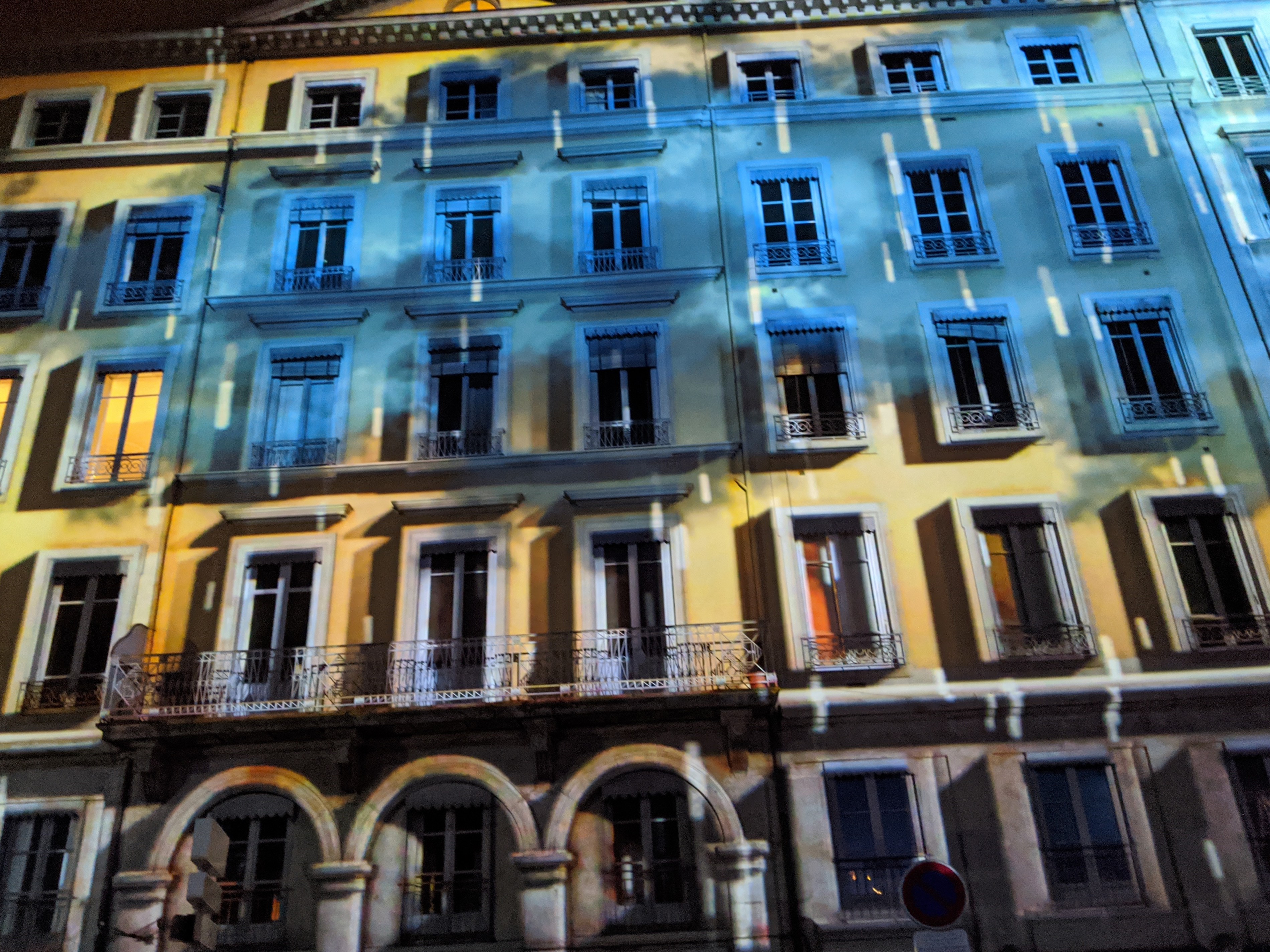
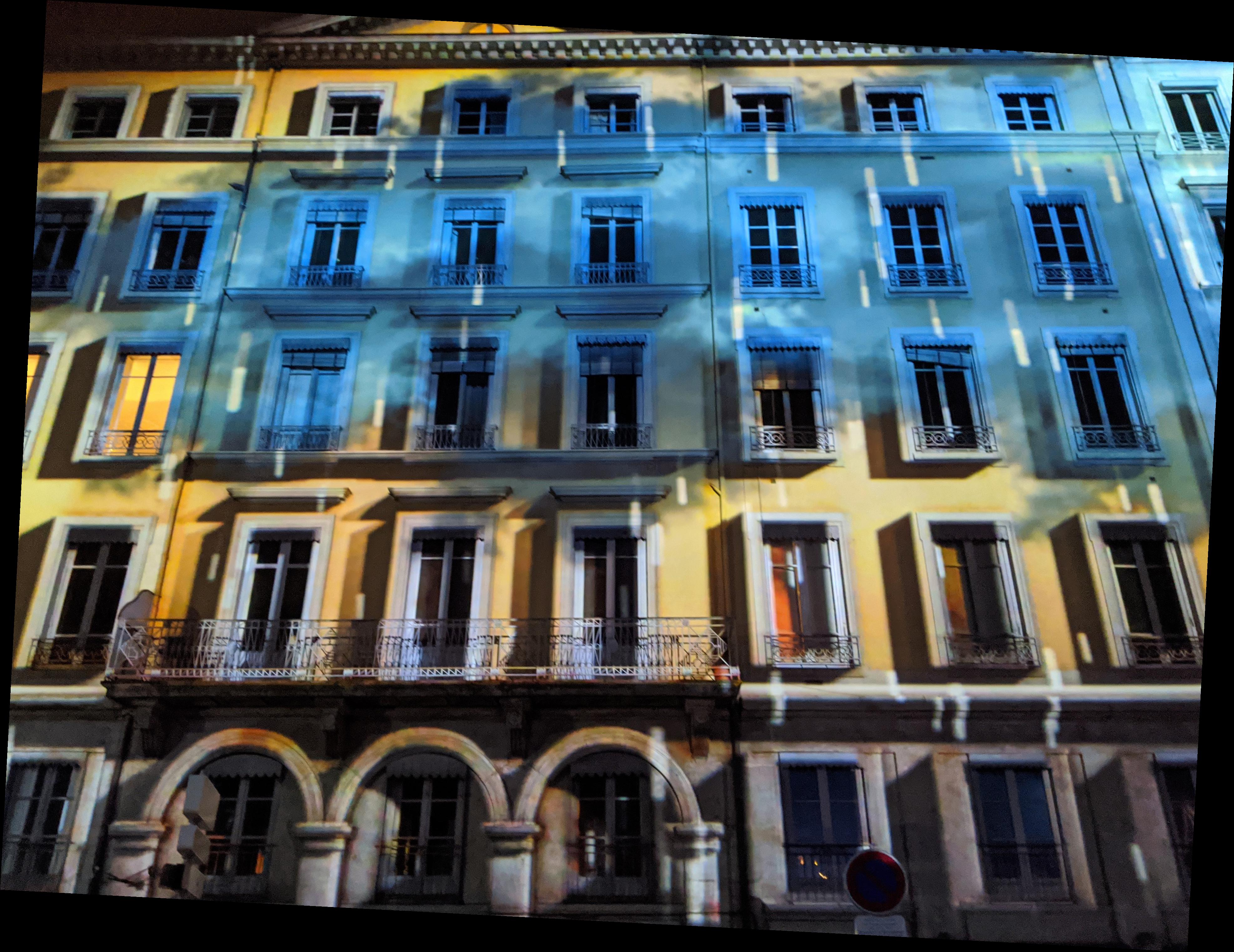
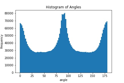
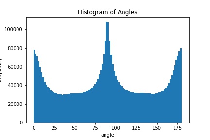
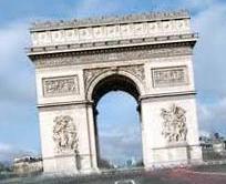
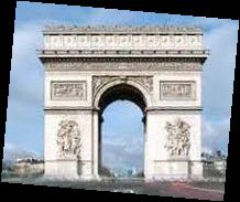
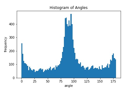
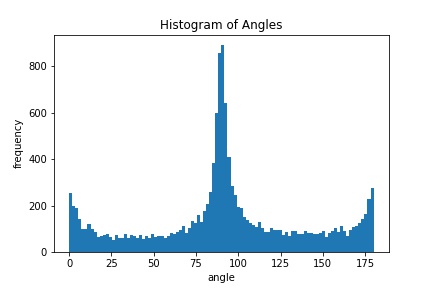
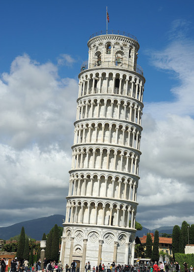
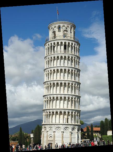
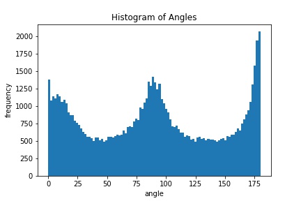
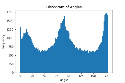
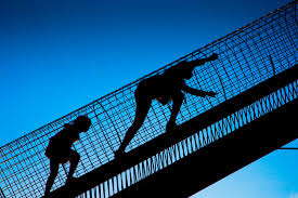
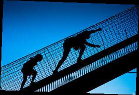
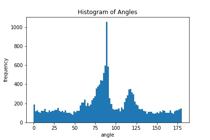
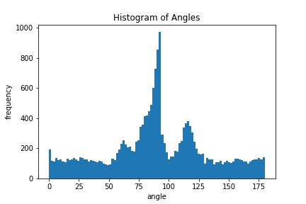
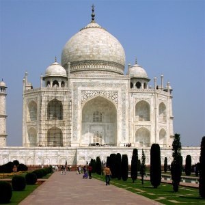
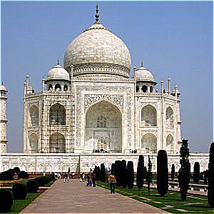
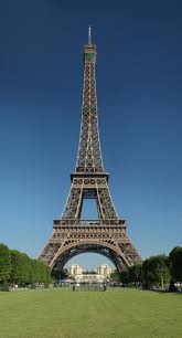
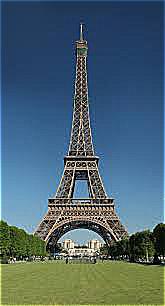
1.3 Image Straightening

For the following images, the first picture is the original image, the second picture is the rotated image, the third picture is the histogram of the original image, and the fourth picture is the histogram of the rotated image. Some values in the histogram were removed, if convolution with both [[1, -1]] and [[1], [-1]] resulted in a value less than 0.05 at the point, as I registered that as no edge. Though the results were good, the last image didn't orient properly, as there are conflicting lines in the image. Looking at the net, it's oriented diagonally, but the springs along the bottom are oriented vertically. Additionally, after cropping, the man in the middle of the image becomes the focus, and it's unclear how to best align this man in isolation.

Part 2

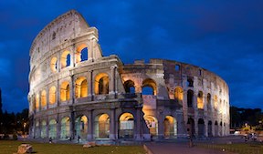
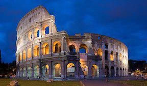
2.1 Image Sharpening

By adding the first laplacian value three times to the gaussian blurred image, I was able to successfully sharpen the images. In the third set of images of the colosseum, I blurred it and tried to implement the sharpening method to see how it would perform. Most notably, performing the operation made the lines of the colosseum darker, but the image didn't feel any more detailed, as this operation cannot create data from nothing.

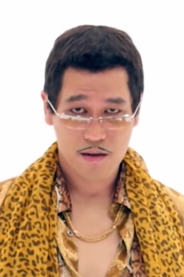
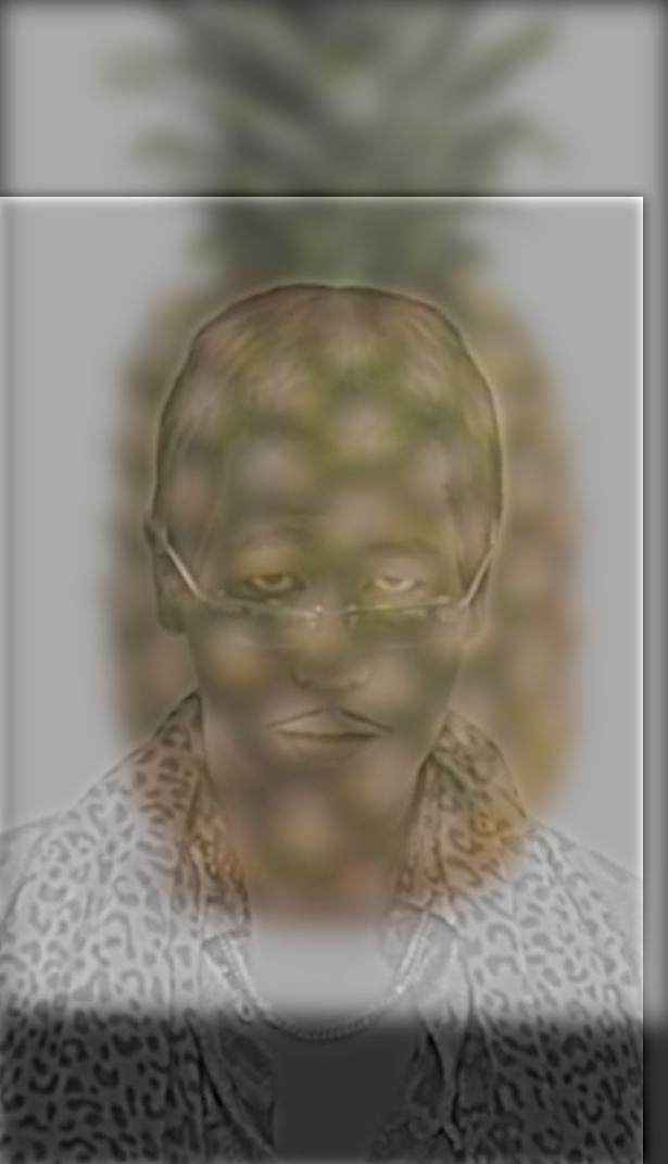
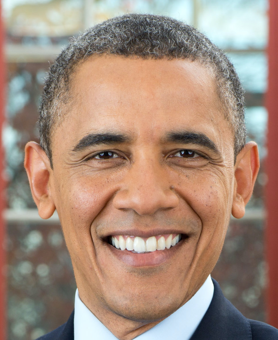
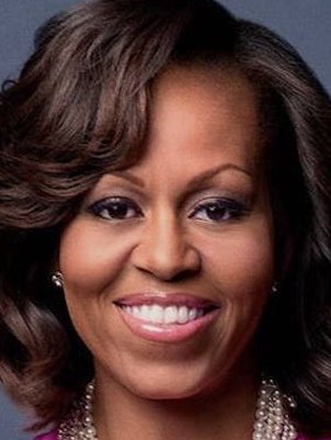
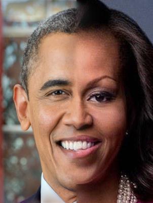
2.2 Hybrid Images

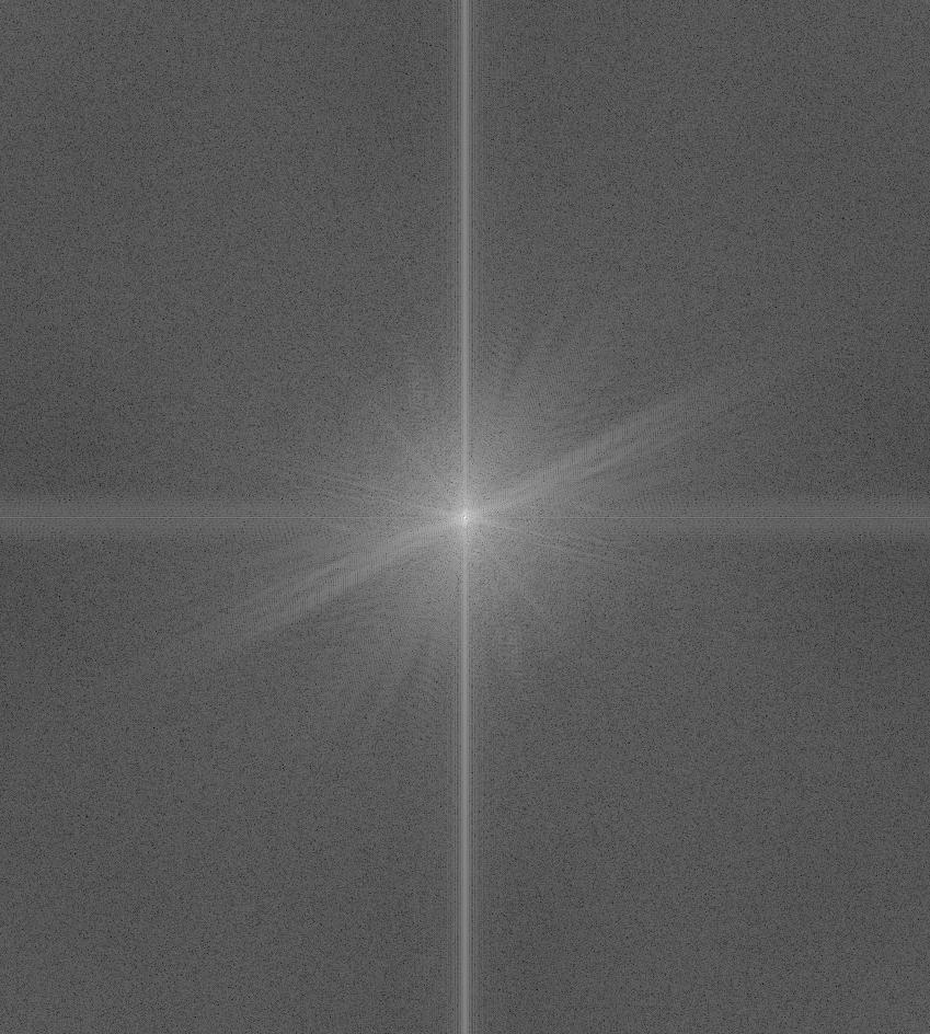
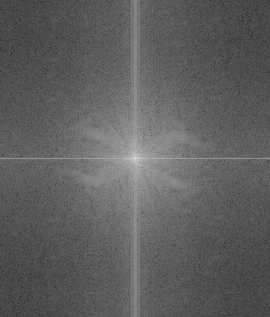
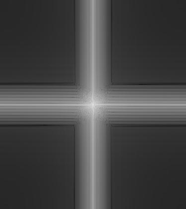
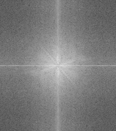
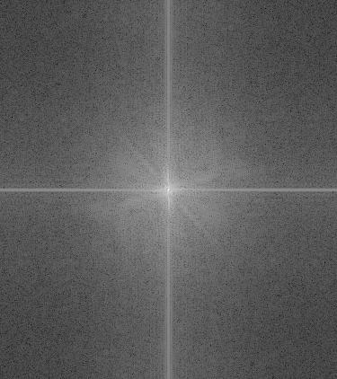
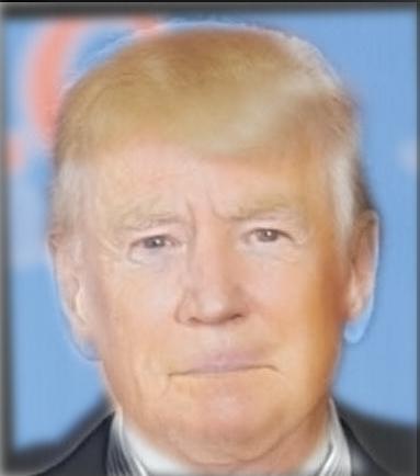
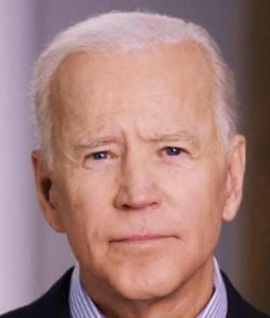
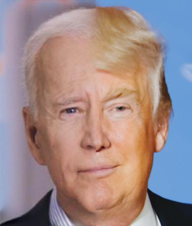
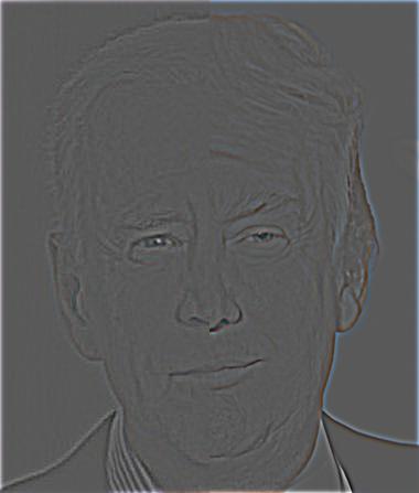
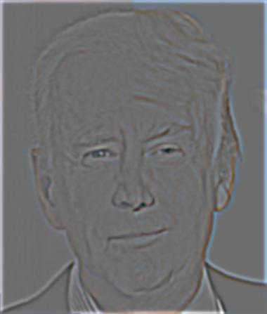
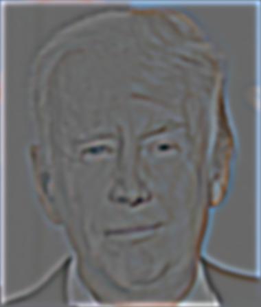
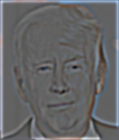
Below are a set of hybrid images that I computed. My favorite result is the hybrid of trump and biden, which I show the grayscale fourier domains for. The third and fourth images are the original fourier domains of the trump and biden images. The fourth and fifth images are the low frequency of the trump image and the high frequency of the biden image. Lastly, the sixth image is the combined result of summing the fourth and fifth images.

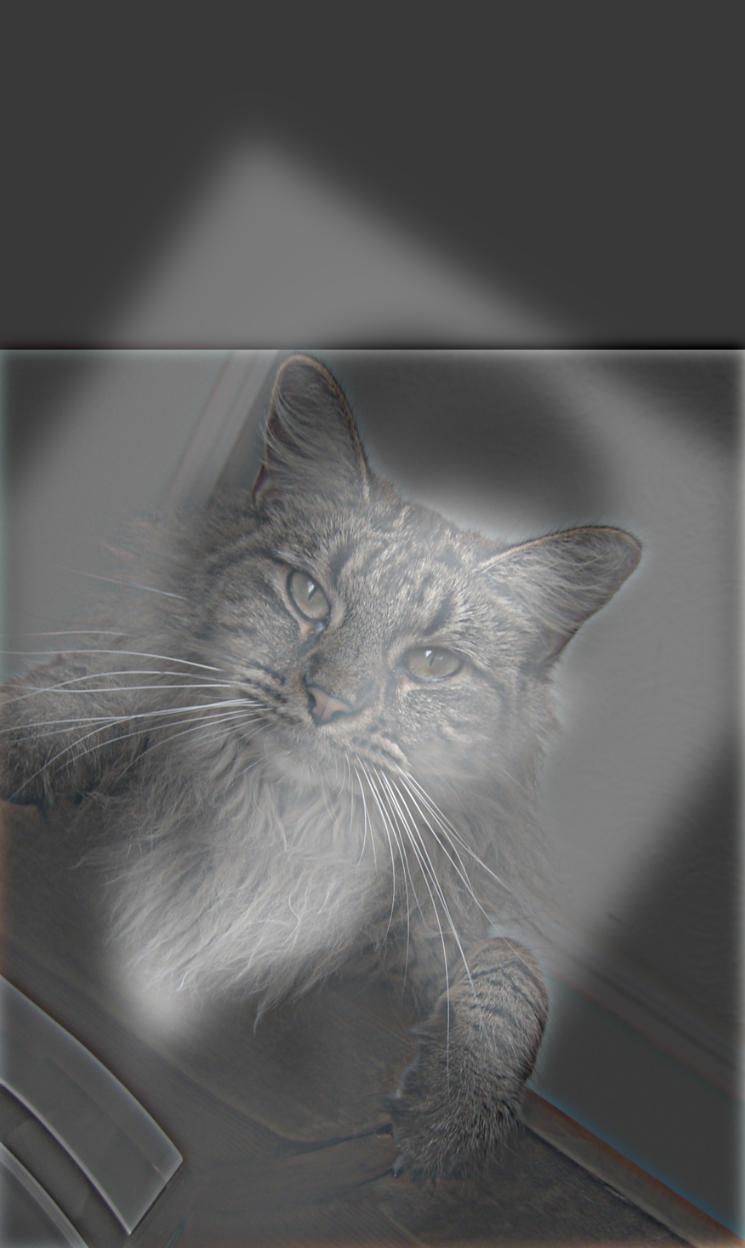
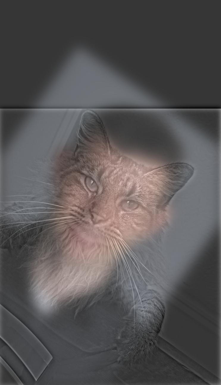
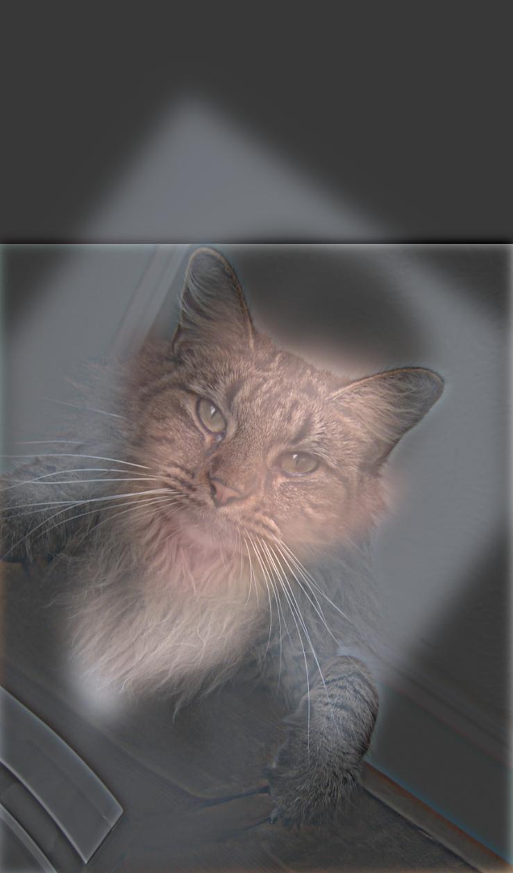
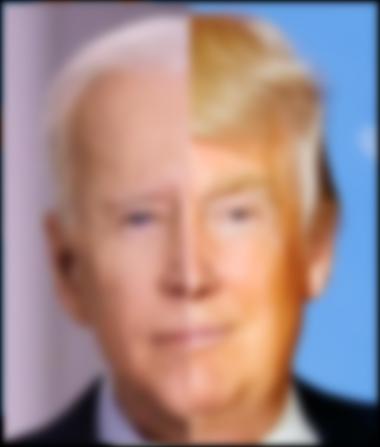
For the bells and whistles, I added color to enhance the effect. The third image is the result of making both images grayscale, the fourth image is the result of making of low frequency image grayscale, and the fifth image is the result of making the high frequency image grayscale. It seems the best results come from making the high frequency image grayscale.

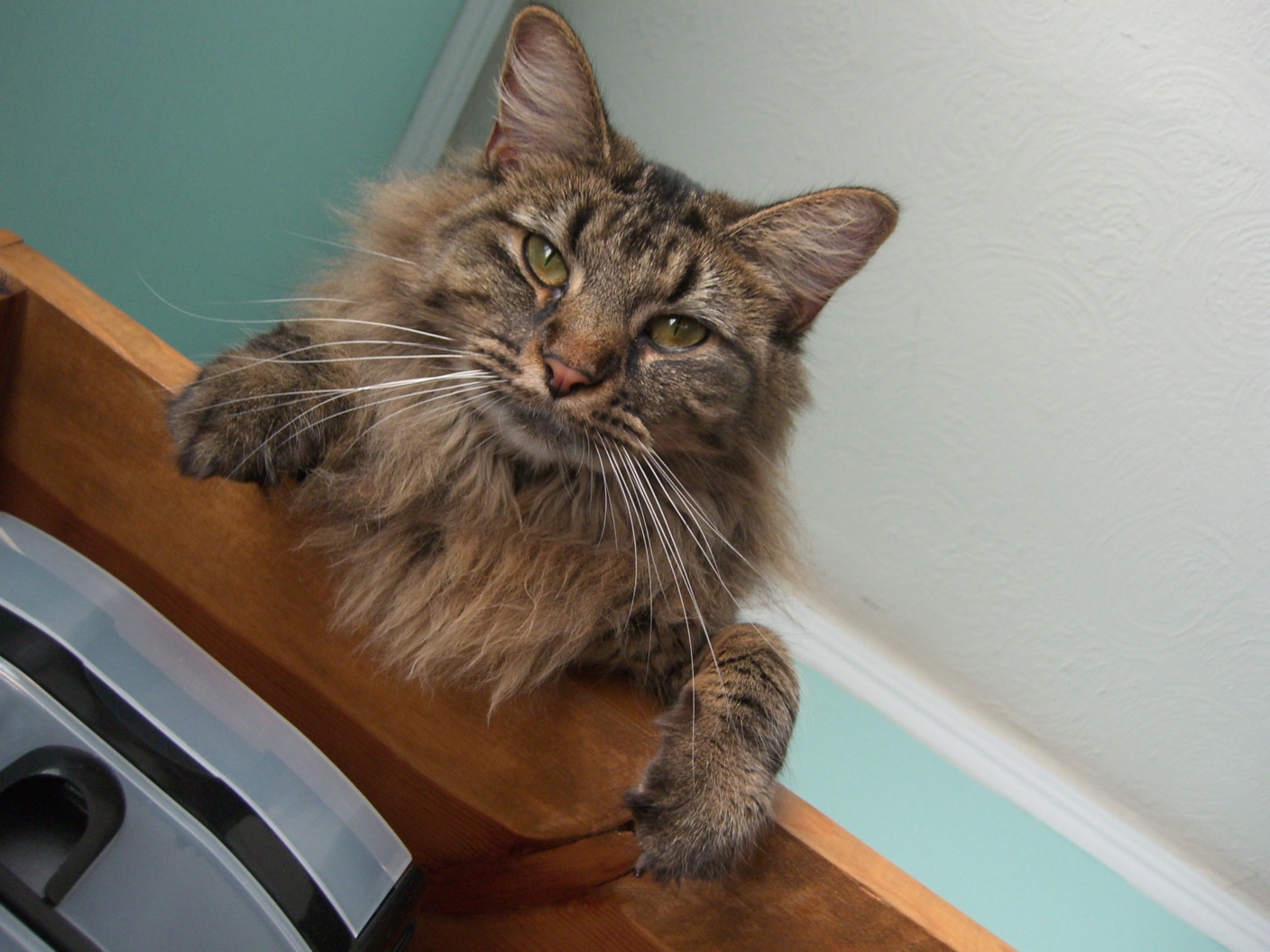
This image failed to blend well, seemingly because their features were too distinct and different to merge. The notable aspects of both images are the intricacies of their high frequency components, so naturally, removing the high frequency components of one while leaving those of the other wouldn't create a good blend.

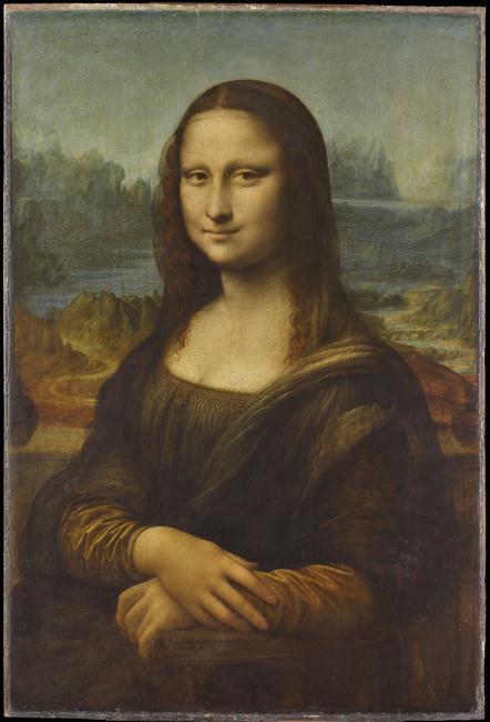
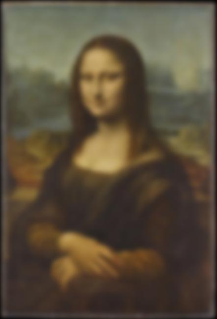
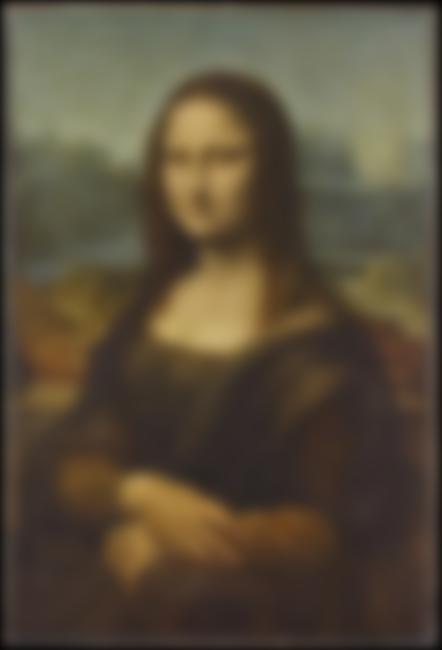
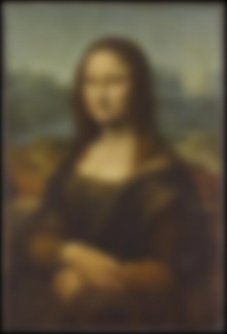
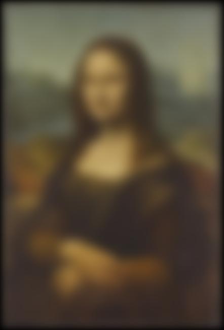
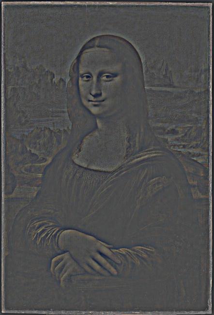
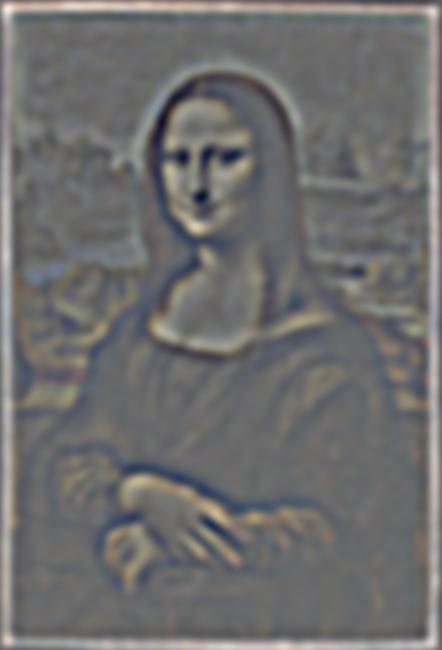
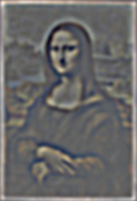
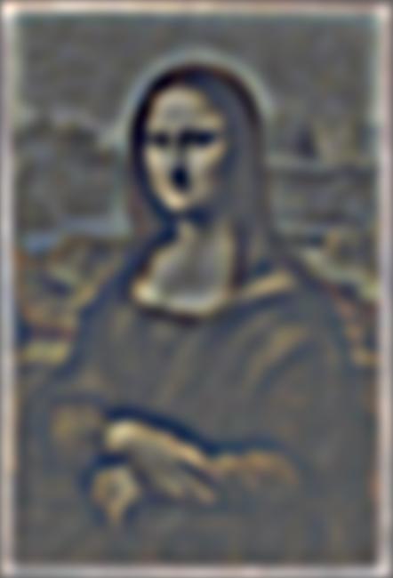
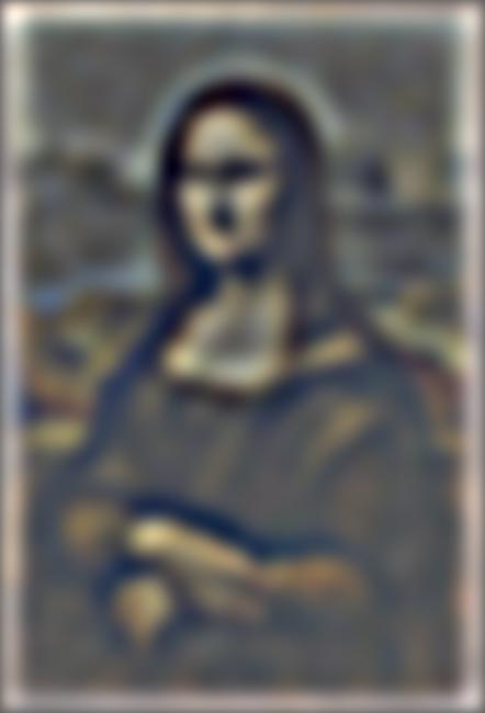
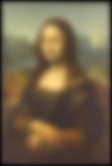
2.3 Gaussian and Laplacian Stacks

The first row is the gaussian stack for Mona Lisa, while the second row is the laplacian stack.

2.4 Multiresolution Blending

For the bells and whistles, I added color to enhance this effect, and I showed the breakdown for the biden + trump image, because it was my favorite result for this blending as well.