CS 194: Image Manipulation and Computational Photography, Fall 2020
Project 2: Fun with Frequencies
Rami Mostafa, cs194-26-abo
Overview
For this project, I got to experiment with editing photos by manipulating different levels of frequencies. This allowed for behaviors such as detecting edges, straightening images, creating hybrid images, and blending images together seemlessly.
Part 1: Fun with Filters
Part 1.1: Finite Difference Operator
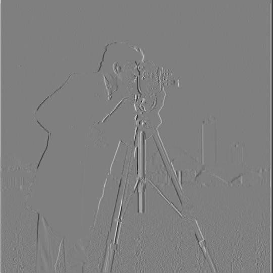
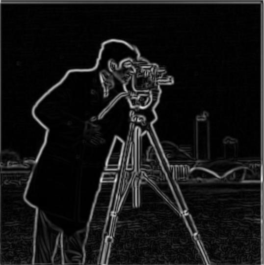
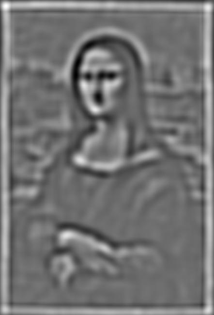
For this section, I simply created dx and dy, and convolved each of them witht the original cameraman image to get the partial derivatives. With the partial derivatives, I computed the gradient magnitude by taking the square root of the sum of the partial derivatives squared. THe result seemed to be a very noisy edge detector.
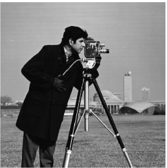 Original Cameraman Image
|
 Partial Derivative of Cameraman (dx)
|
 Partial Derivative of Cameraman (dy)
|
|
 Gradient Magnitude of Derivatives
|
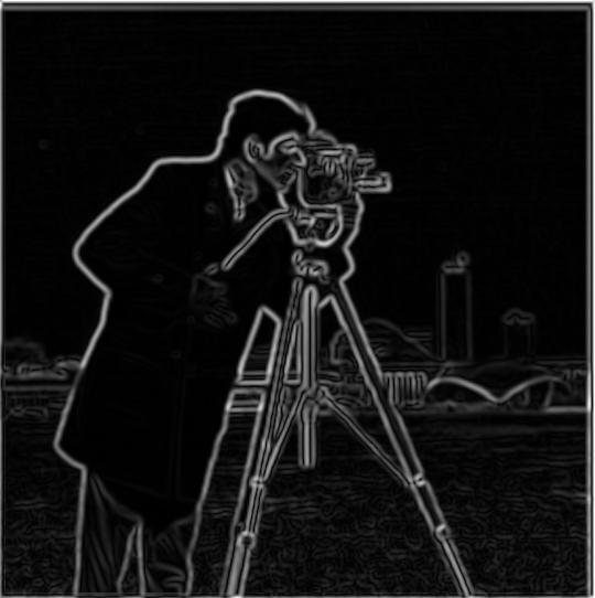
Part 1.2: Derivative of Gaussian (DoG) Filter
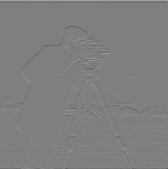
For this section, we did the same process as in section 1.1, but began by first blurring the image.
 Gradient Magnitude of Blurred Image
|
The main difference here is that this is a much smoother edge detector than the one computed in section 1.1. By blurring the image, the loss of detail causes certain areas in the image such as the grass to be detected less in the partial derivatives. This is because the blurring causing the pixels to seemingly blend together, and because all of the grass has similar RGB values, the edges among the grass seem to disappear. However, much more explicit edges such as the edge between the person and the sky will require a lot more blurring to obscure. Therefore, we can still see these types of edges well represented in the gradient. As a result, we reduce the noise detected from part 1.1 and are able to more cleary see the significant edges in the image.
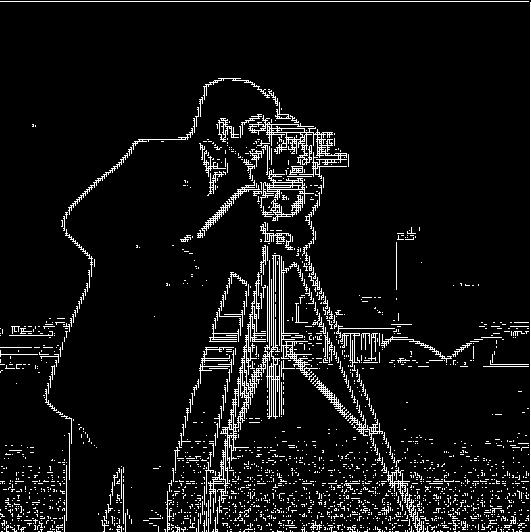
We also computed the gradient magnitude of the blurred image via a different process where instead of blurring the original image, we computed the partial derivatives of the gaussian filter, and convolved those results with the original image.
|
Original Image
|
 Partial Derivative of Gaussian Filter (dx)
|
 Partial Derivative of Gaussian Filter (dy)
|
 Gradient Magnitude Image
|
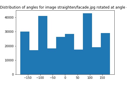
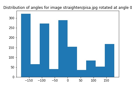
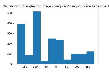
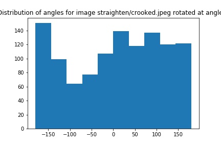
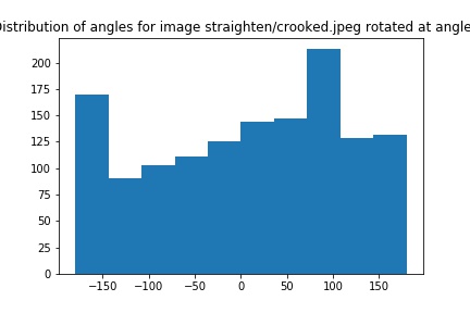
Part 1.3: Image Straightening
For this section, I used what we had learned in the previous sections to construct an algorithm capable of straightening any image with clear straight lines. For each image, I would rotate them along the range of -10 to 10 degrees. For each rotation, I ran an algorithm that computed a score that would increase with the more gradient angles that the rotated image has that is a multiple of 90 (0, 90, -90, 180, -180, etc.). After testing each angle, I simply rotated the image by the angle that produced the max score to get the straightened image.
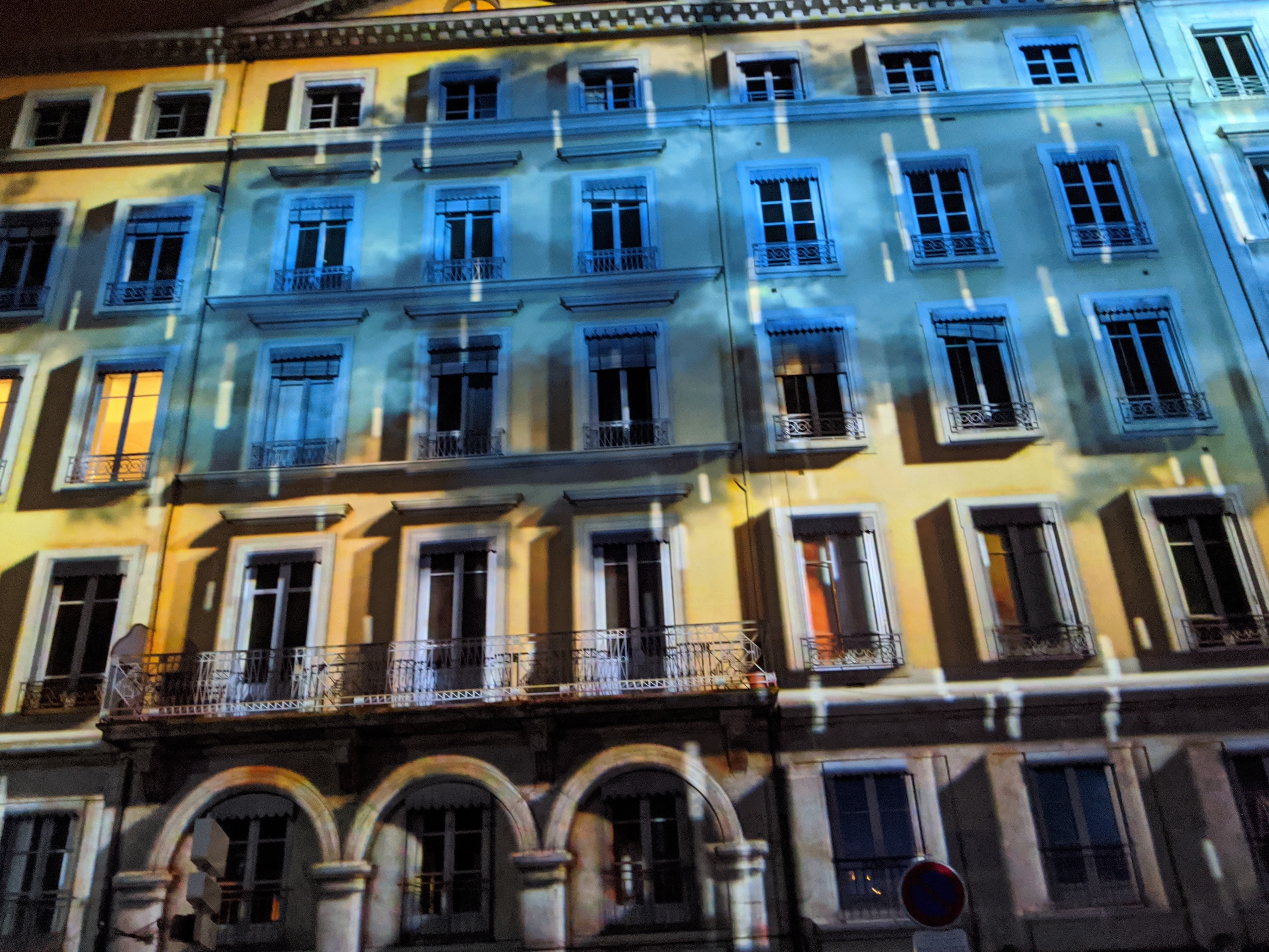 Original Facade Image
|

|
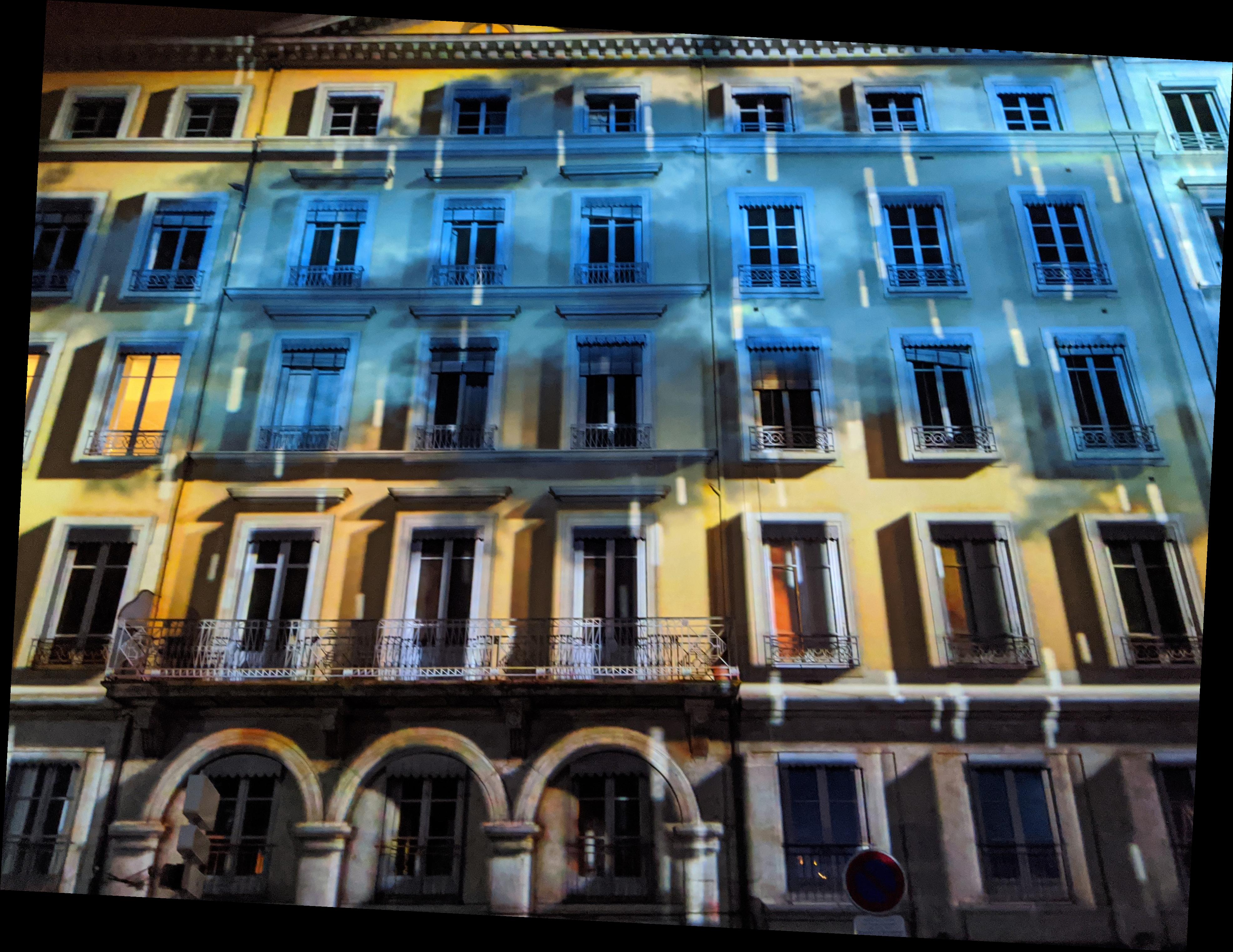 Straight Facade Image (Rotated -3 degrees)
|
|
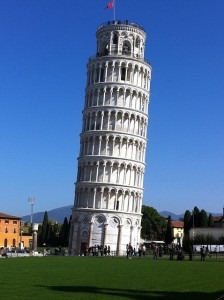 Original Pisa Image
|
|
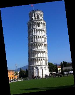 Straight Pisa Image (Rotated 7 degrees)
|
|
As stated before, this algorithm only applies to images with clear straight lines, especially those that are meant to be horizontal or vertical. As a result, this algorithm may lead to some failure cases such as the one below due to no clear horizontal or vertical lines at any rotation.
 Original Curved Building Image
|
|
 Rotated Curved Building Image (Rotated -5 degrees)
|
|
Part 2: Fun with Frequencies
Part 2.1: Image "Sharpening"
In this section, I was able to manipulate the high and low frequencies of an image to produce images of sharper detail than the original image. To achieve this result, I would apply a gaussian filter to the image to produce a resulting image with only low frequencies. Then I would subtract the low frequency image from the original to get an image of only high frequencies. Finally, to add the extra sharpness, I simply added high frequencies back to the original image to further sharpen the details.
However, this process can be replicated via a single convolution of the original image and a linear expression of the unit impulse and the gaussian filter. This was the process used to achieve the results below.
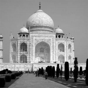 Original Taj Mahal Image
|
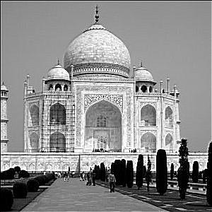 Sharpened Taj Mahal Image
|
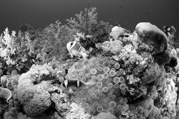 Original Coral Reef Image
|
 Sharpened Coral Reef Image
|
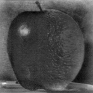
Using this process of sharpening images, I tried to take an already sharp image, blur it, and attempt to see if I could recreate the originally sharp image.
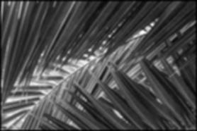
 Original Sharp Leaves Image
|
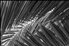
 Blurred Leaves Image
|
 Resharpened Leaves Image
|
As can be seen above, we cannot recreate the original image by sharpening a blurred version of the original. This is because blurring an image results in a significant loss of information that cannot be used or rediscovered. Therefore, it is impossible to recreate the origina image since we do not have all of the necessary information. We can produce an image that is sharper than the blurred version, but will never be able to reproduce the original image.
Part 2.2: Hybrid Images
For this section, I constructed a process of aligning two images (I chose to align images using the eyes of the subjects in the two images), and combining the low frequencies of one aligned image with the high frequencies of the other to create what we refer to as a hybrid image. This image tends to appear as either the image used for the low or high frequencies depending on how far away a person physically is from the hybrid image.
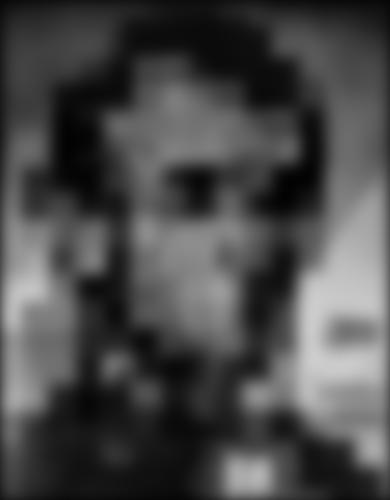
 Original Nutmeg (High Frequency)
|
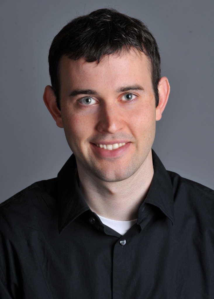 Original Derek (Low Frequency)
|
 Nutmeg-Derek Hybrid Image
|
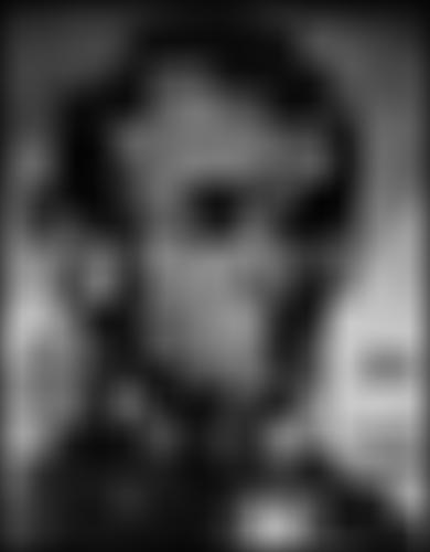
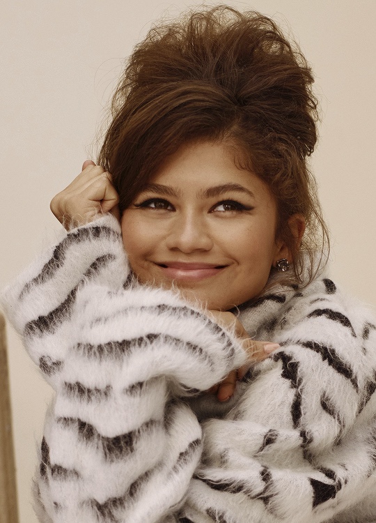 Original Happy Zendaya (High Frequency)
|
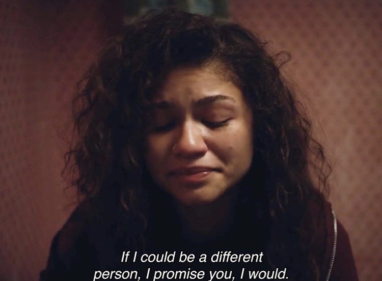 Original Sad Zendaya (Low Frequency)
|
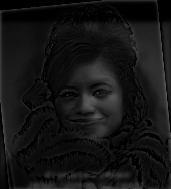 Nutmeg-Derek Hybrid Image
|
Below is a more explicit showcase of the process on the hybrid image of a wounded Detective Pikachu, and the classic suprised pikachu meme.
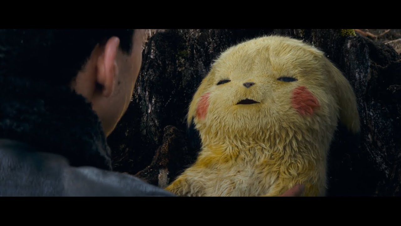 Original Wounded Pikachu Image
|
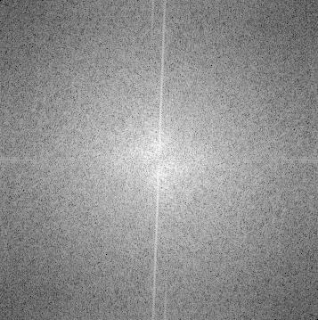
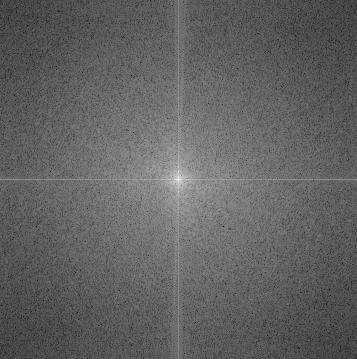
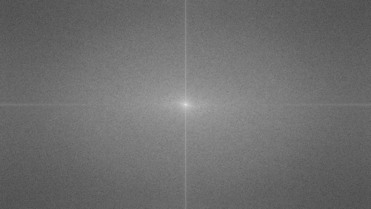 FFT Domain of Wounded Pikachu
|
 Original Surprised Pikachu Image
|
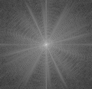 FFT Domain of Surprised Pikachu
|
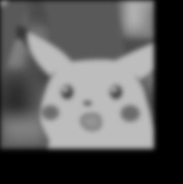
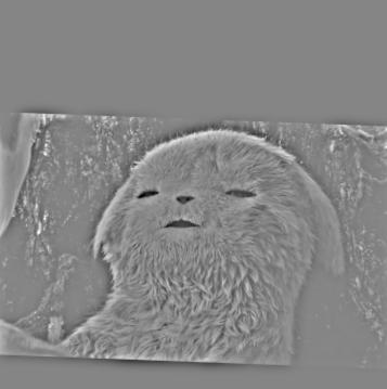 High Frequencies of Wounded Pikachu
|
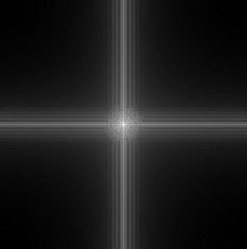
 FFT Domain of High Frequencies
|
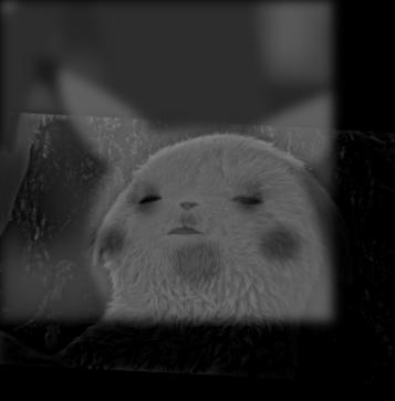
 Low Frequencies of Surprised Pikachu
|
 FFT Domain of Low Frequencies
|
 Wounded-Surprised Pikachu Hybrid
|
 FFT Domain of Hybrid Image
|
Additionally, there may be some cases in which this algorithm does not produce the best result. I found one of these failure cases when trying to create a hybrid image of Spongebob Squarepants and Squidward Tentacles. Many details of both images can be seen at any distance. I believe this case failed due to the large difference in shape of the two subjects I attempted to create a hybrid image of. Failing to align the subjects well seems to result in not being able to create this hybrid effect.
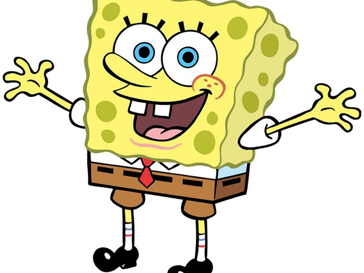 Original Spongebob (High Frequency)
|
 Original Squidward (Low Frequency)
|
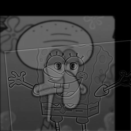 Spongebob-Squidward Hybrid Image
|
Part 2.3: Gaussian and Laplacian Stacks
In this section I constructed a gaussian and laplacian stack for a given image. To construct the gaussian stack, I simply applied a 40x40 gaussian filter with an initial sigma of 5 to the input image. This creates the first image in our gaussian stack. Then, I applied the same gaussian filter to the input image, but with a doubled sigma value. As a result, the effect of the gaussian filter would increase with each successive layer of the gaussian stack. Once the gaussian stack was created, I simply subtracted each image in the stack from the image immediately before it to construct the laplacian stack.
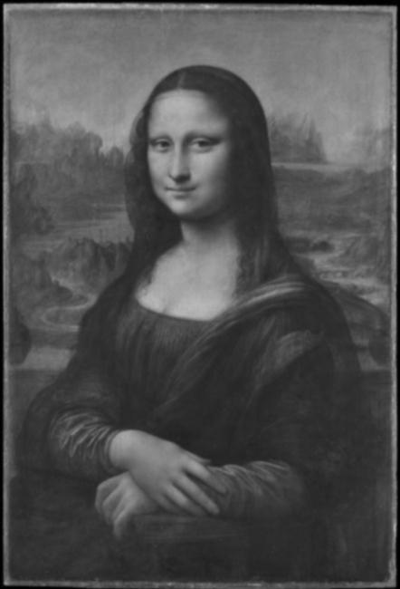
 Gaussian Stack Level 0 (Original)
|
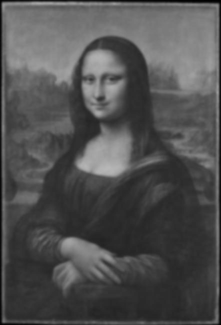
 Gaussian Stack Level 1
|
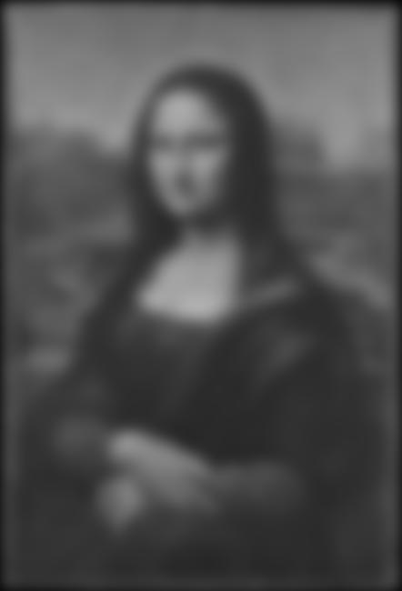
 Gaussian Stack Level 2
|
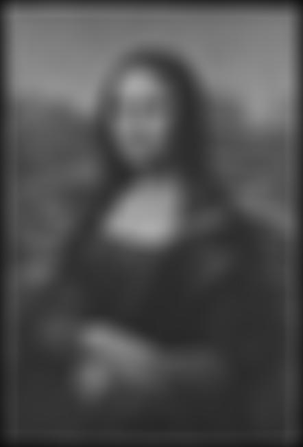
 Gaussian Stack Level 3
|
 Gaussian Stack Level 4
|
 Gaussian Stack Level 5
|
 Original Image
|
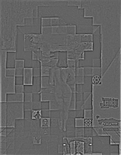
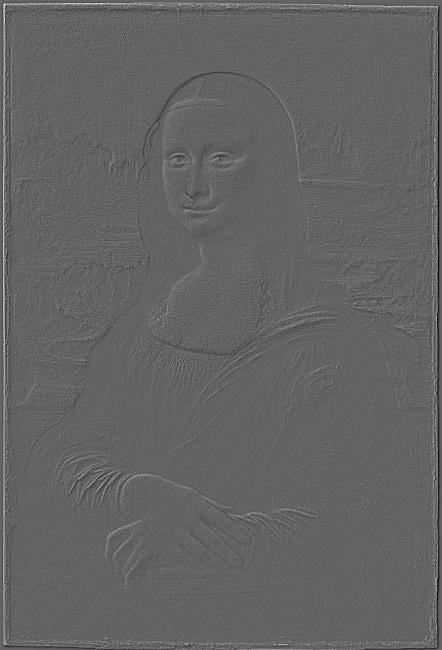
 Laplacian Stack Level (1 - 0)
|
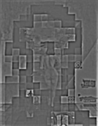
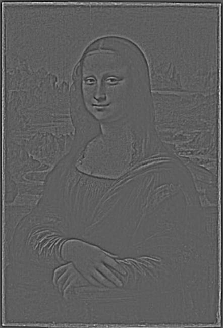
 Laplacian Stack Level (2 - 1)
|
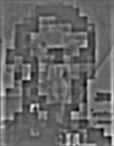
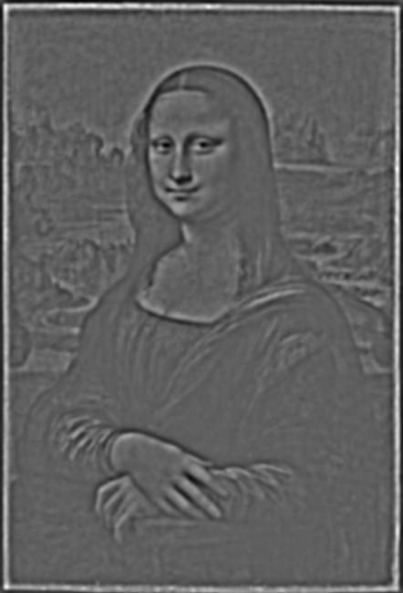
 Laplacian Stack Level (3 - 2)
|
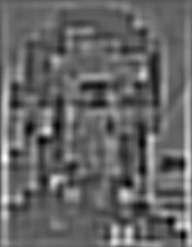
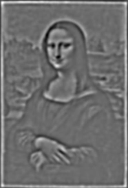
 Laplacian Stack Level (4 - 3)
|
 Laplacian Stack Level (5 - 4)
|
 Gaussian Stack Level 0 (Original)
|
 Gaussian Stack Level 1
|
 Gaussian Stack Level 2
|
 Gaussian Stack Level 3
|
 Gaussian Stack Level 4
|
 Gaussian Stack Level 5
|
 Original Image
|
 Laplacian Stack Level (1 - 0)
|
 Laplacian Stack Level (2 - 1)
|
 Laplacian Stack Level (3 - 2)
|
 Laplacian Stack Level (4 - 3)
|
 Laplacian Stack Level (5 - 4)
|
Part 2.4: Multiresolution Blending (a.k.a. the oraple!
For this final section, I explored how we can use gaussian and laplacian stacks to apply seemless blends of some completely different images. To do this, I first reshape a pair of images so they they are the same shape and contain the subjects I intend to blend. Then I compute the gaussian and laplacian stacks for each of these reshaped images. After, I construct a mask that is also the same shape, and contains only 1s and 0s. I also construct a gaussian stack for the mask as well. Then, for each element in each laplacian stack (we can call them LA and LB for short), and for each mask in the mask's gaussian stack (we can call it M) I compute LA * M + LB * (1 - M) to create a stack of blended images. Finally, I sum over the stack to create my final blended image.
 Original Apple Image
|
 Original Orange Image
|
 Linear Mask
|
 Blended Orapple Image
|
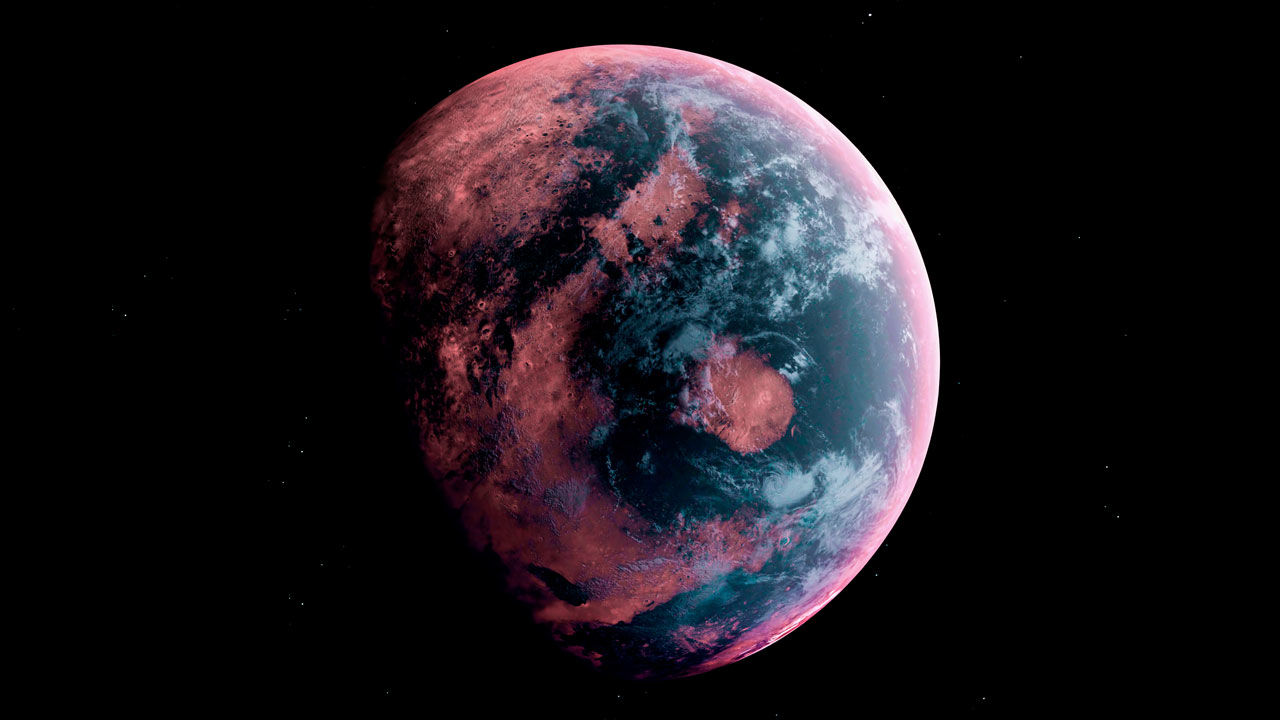 Original Planet Image
|
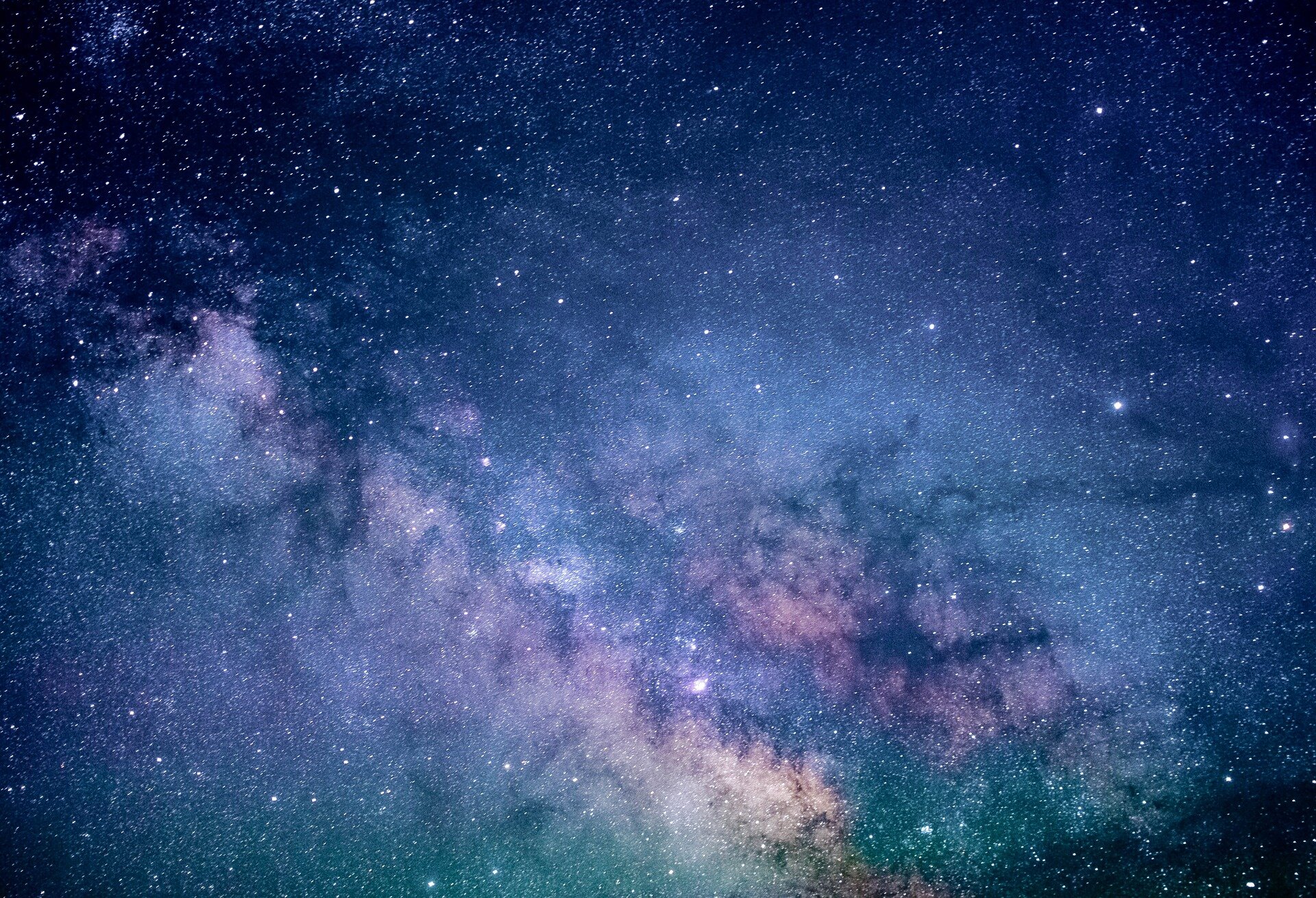 Original Space Image
|
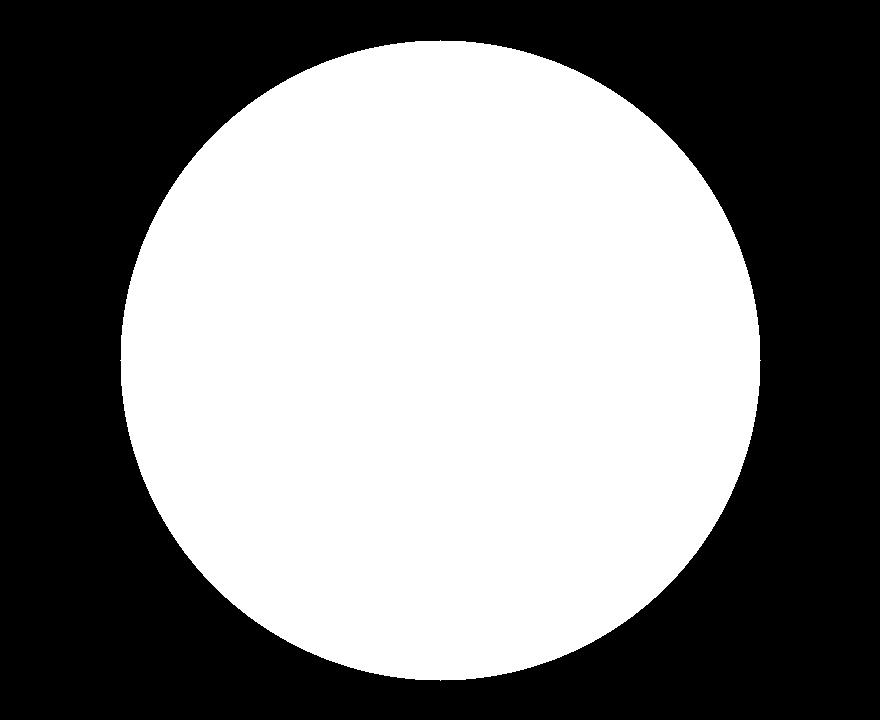 Circle Mask
|
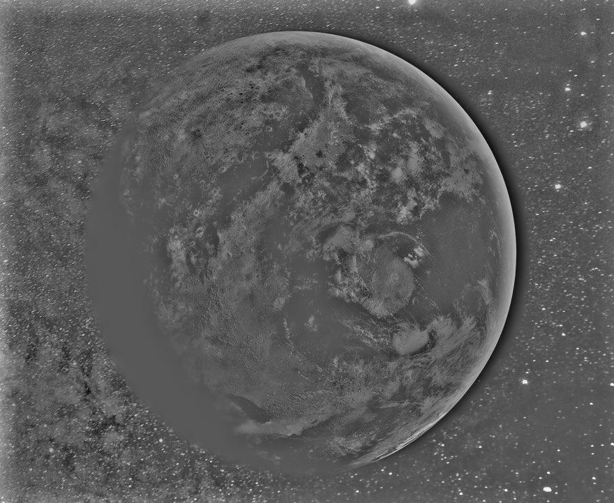 Blended Planet-Space Image
|
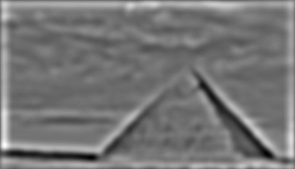
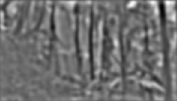
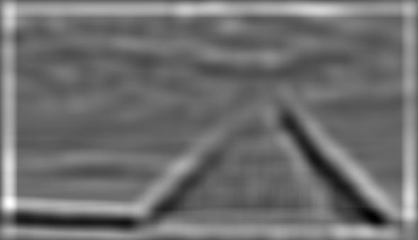
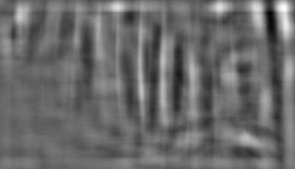
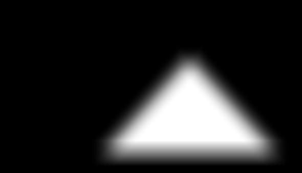
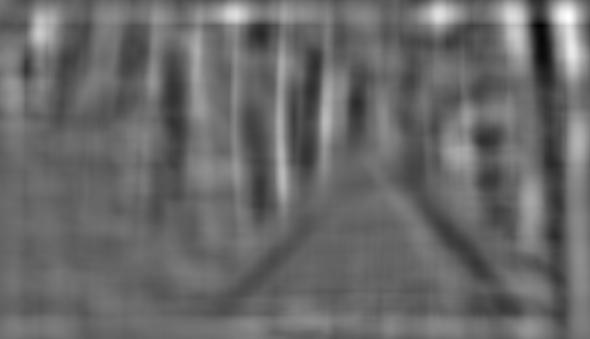
Below we can see a more detailed showcase of the process on the Pyramid and Forest images.
Input Images and Mask
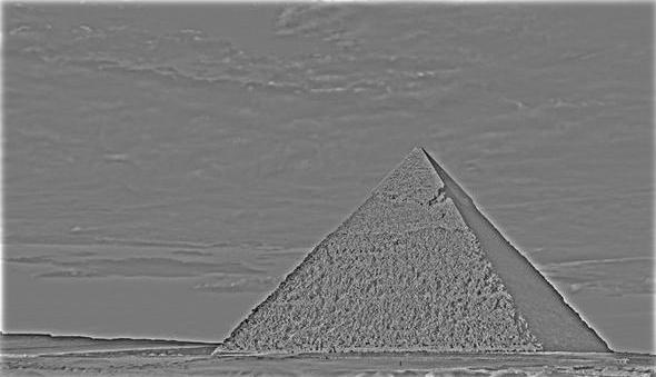
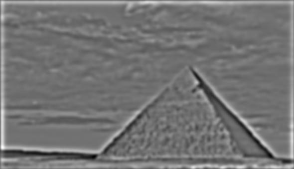
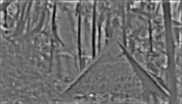
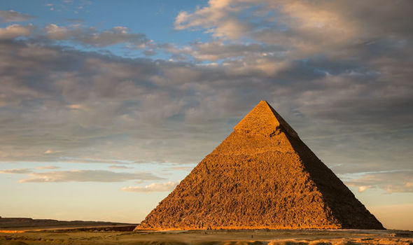 Original Pyramid Image (Level 0)
|
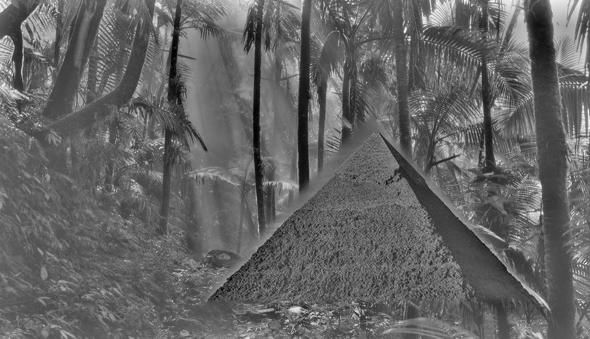
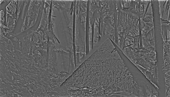
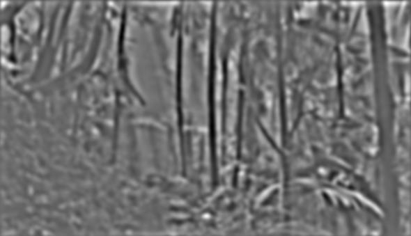
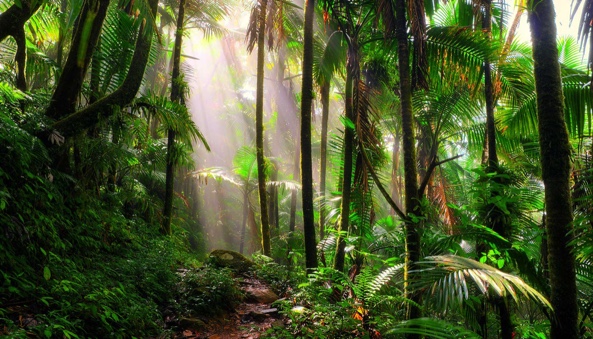 Original Forest Image (Level 0)
|
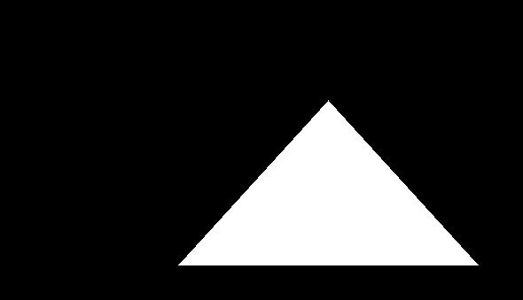 Triangle Mask (Level 0)
|
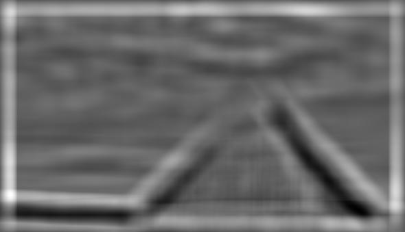
 Blended Image (Sum of blends below)
|
 Laplacian Pyramid Level 1
|
 Laplacian Forest Level 1
|
 Gaussian Mask Level 1
|
 Blended Pyramid-Forest Image Level 1
|
 Laplacian Pyramid Level 2
|
 Laplacian Forest Level 2
|
 Gaussian Mask Level 2
|
 Blended Pyramid-Forest Image Level 2
|
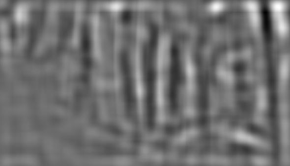
 Laplacian Pyramid Level 3
|
 Laplacian Forest Level 3
|
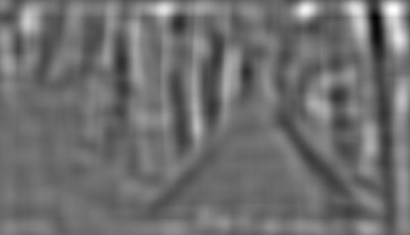
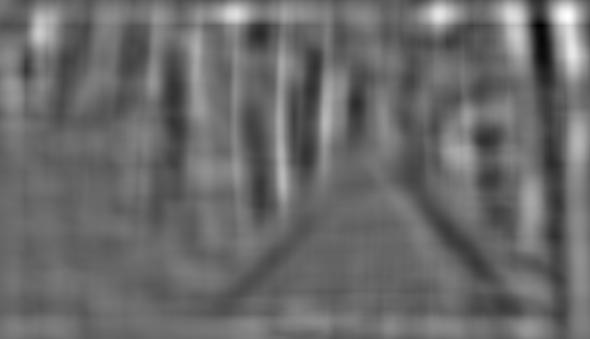
 Gaussian Mask Level 3
|
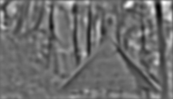 Blended Pyramid-Forest Image Level 3
|
 Laplacian Pyramid Level 4
|
 Laplacian Forest Level 4
|
 Gaussian Mask Level 4
|
 Blended Pyramid-Forest Image Level 4
|
 Laplacian Pyramid Level 5
|
 Laplacian Forest Level 5
|
 Gaussian Mask Level 5
|
 Blended Pyramid-Forest Image Level 5
|
 Laplacian Pyramid Level 6
|
 Laplacian Forest Level 6
|
 Gaussian Mask Level 6
|
 Blended Pyramid-Forest Image Level 6
|