The second project involved using various filtering and blurring techniques in order to alter and enhance images.
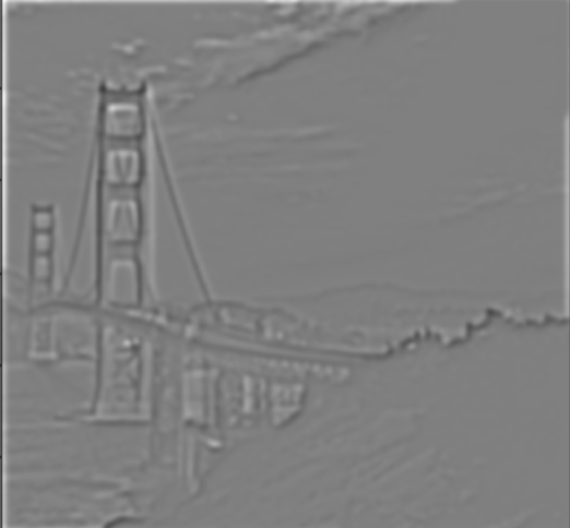
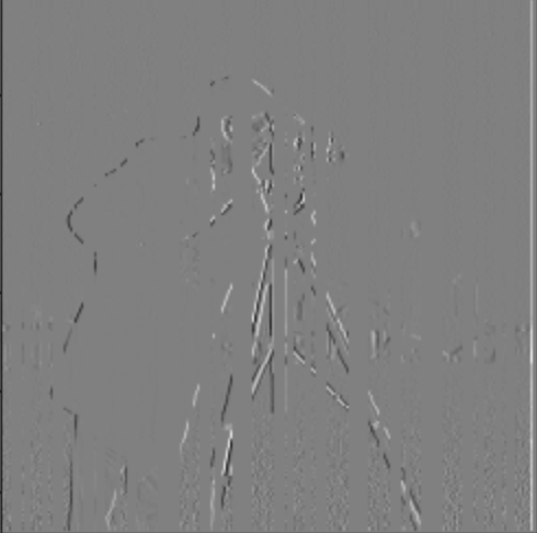
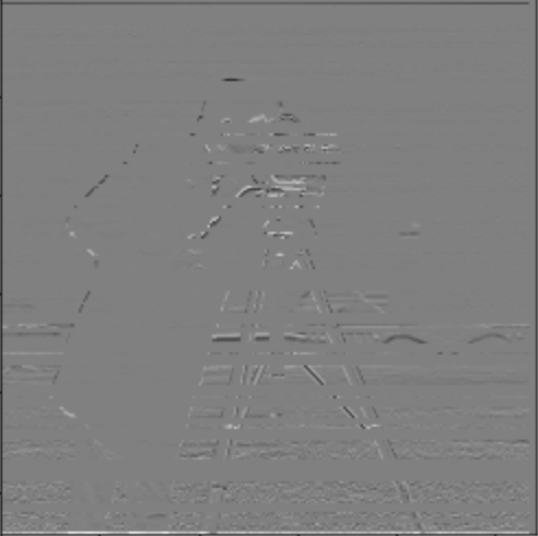
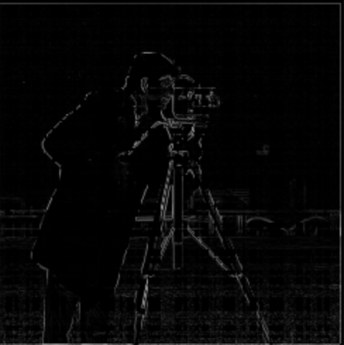
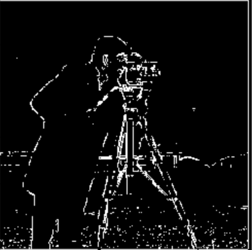
In order to find the edges of the image, we can use the dx kernel [1, -1] and dy [[1], [-1]] to convolve with the original image. With both of these gradient images, we can then compute the gradient magnitdue (sqrt(dx^2 + dy^2)) in order to combine and determine the edge strength in the image. Finally, we can find a magnitude threshold and binarize the image to produce the final edge image.
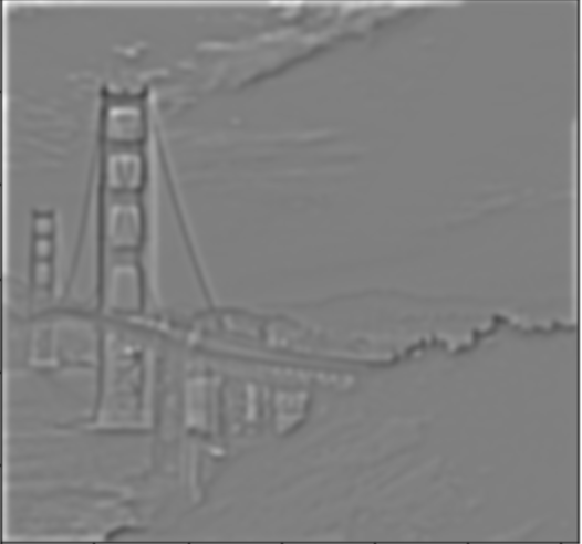
We can apply a gaussian filter first to the cameraman image and then calculate the partial derivatives as in the previous part. The initial blurring will provide better results as it removes some of the higher frequencies. We can see that applying the gaussian blur creates much more defined edges in the gradient magnitudes.
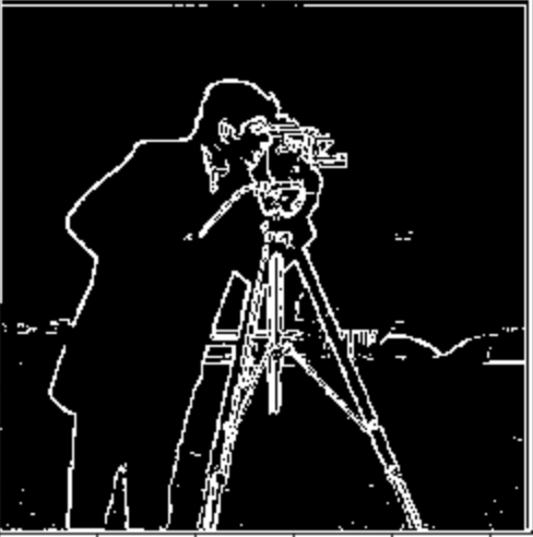
The guassian and derivative convolution operations can be combined into one convolution. We develop a Derivative of Gaussian (DoG) filter and convolve each once with the cameraman image.
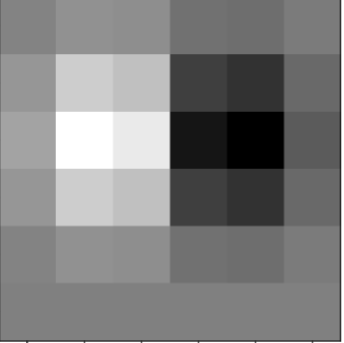

Convolving the above filters and then computing the gradient magnitude image results in the exact same image as using 2 separate operations.
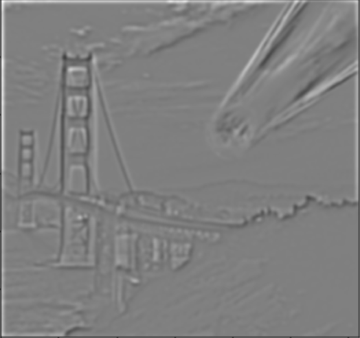
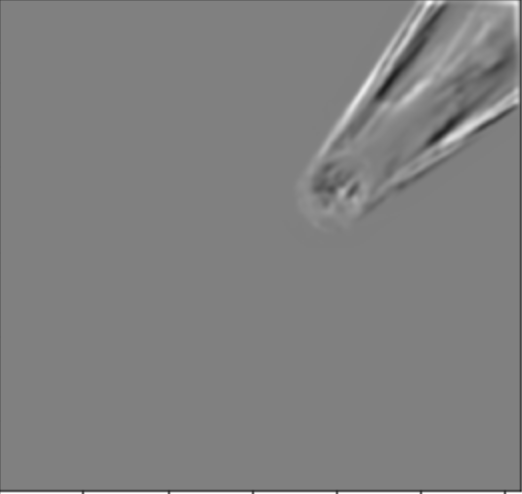
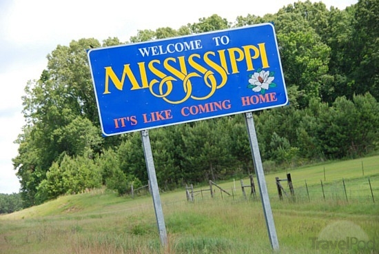
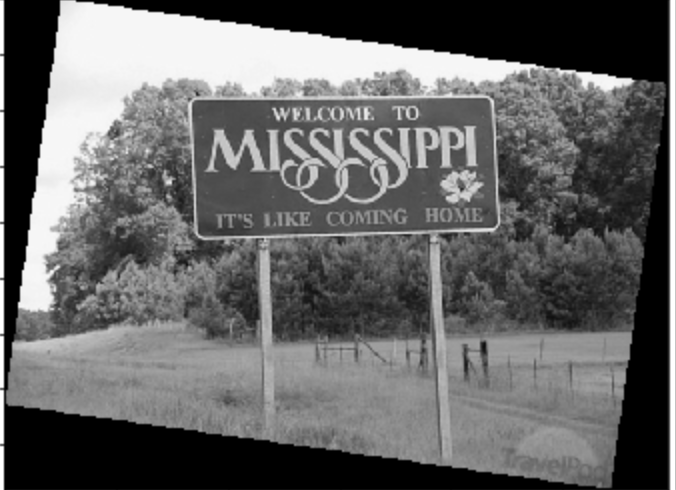
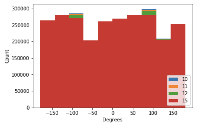
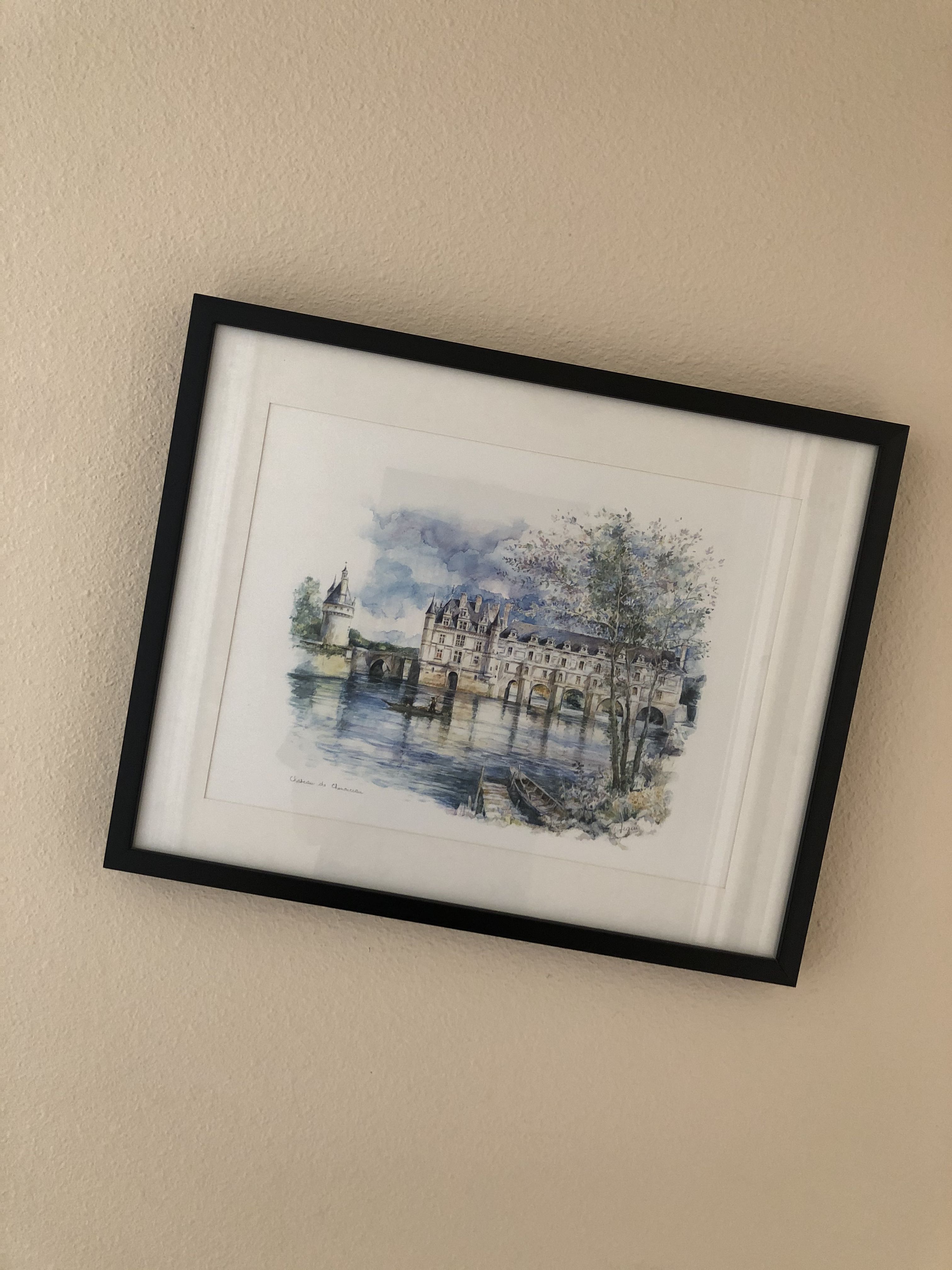
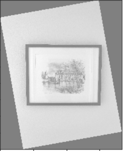
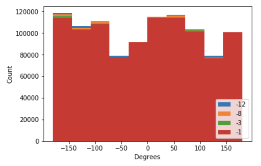
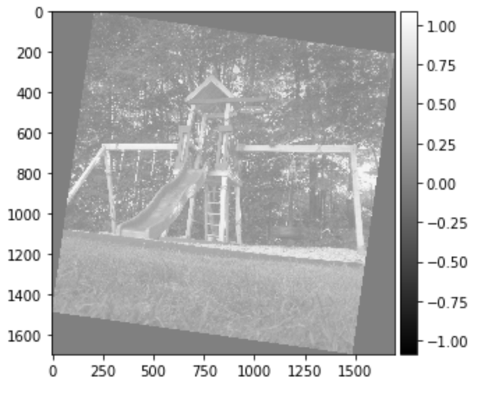
In order to straighten images that are crooked, we need to leverage gradient angles in order to determine which image is straight. A gradient angle is found by finding the arctan of the partial derivatives of an image. A straight image is one that has the highest number of 90 and -90 degree angles in it compared to others. I generated a small subset of possible angles and then generated a histogram of the distribution of gradient angles in each rotated image. I then selected the rotation that yielded the highest number of -90 and 90 degree angles.
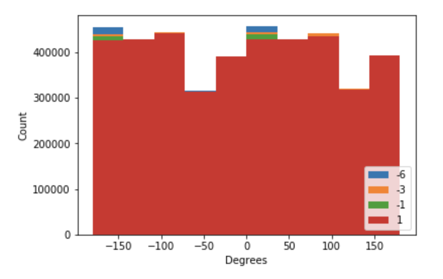
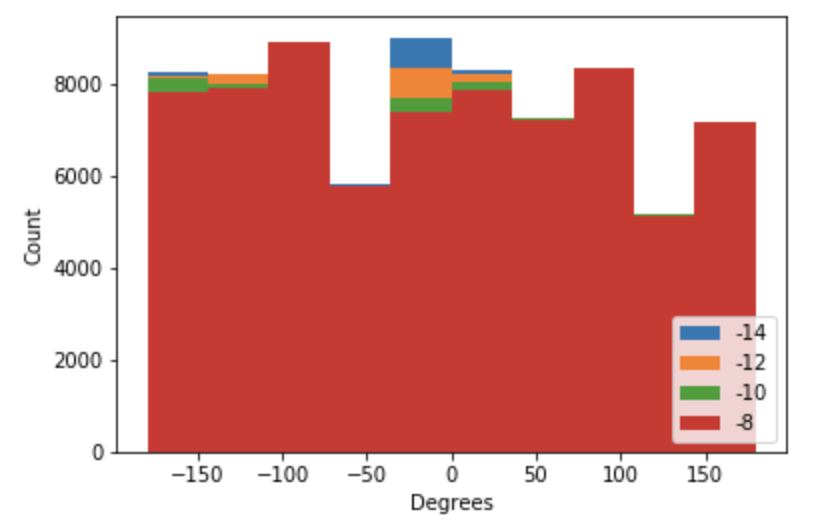
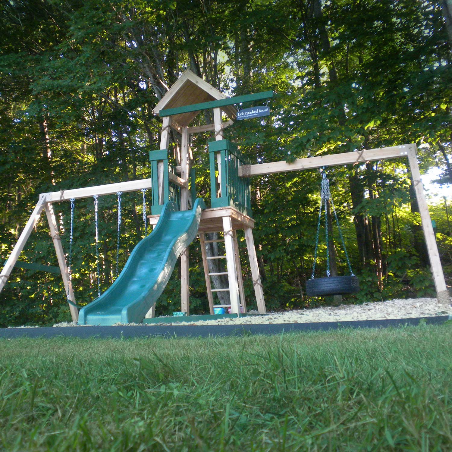
I tried to straighten an image of a swingset on a field. A truly straightened image would just make the horizon of the image straight. But the prominent edges in this image are the angled swing supports and thus looking at the distribution of angles, the best fit angle actually aligns the swing supports to be straight and not the picture horizon.
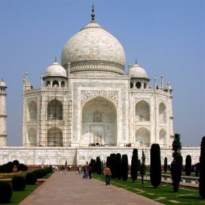
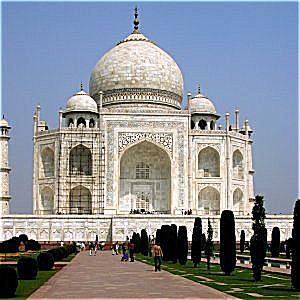
In this part, we had to sharpen blurry images so that to the human eye it looks clearer and crisper. In order to fool the human eye, the amount of high frequency boosting has to be closely regulated.
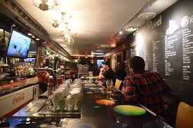


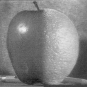
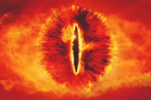
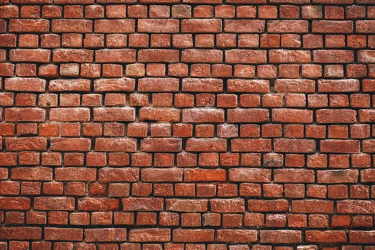
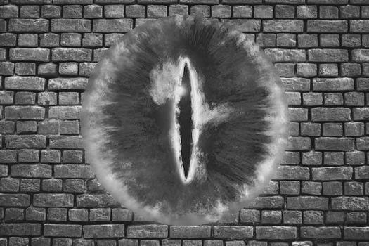
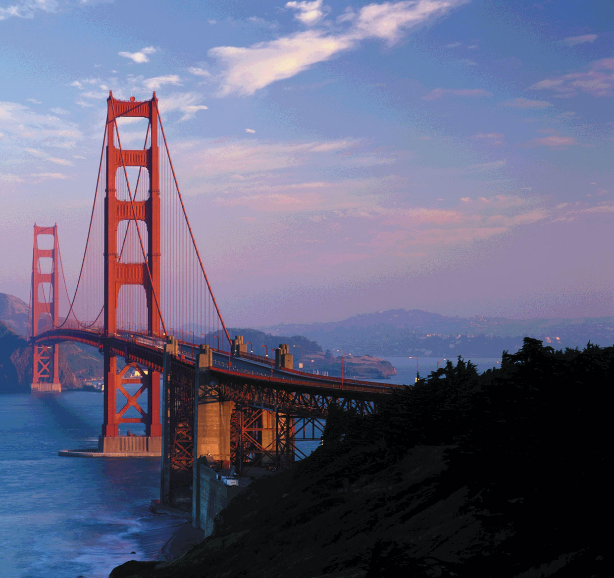
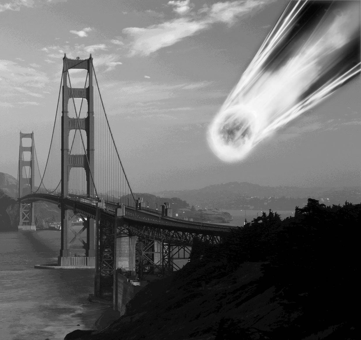
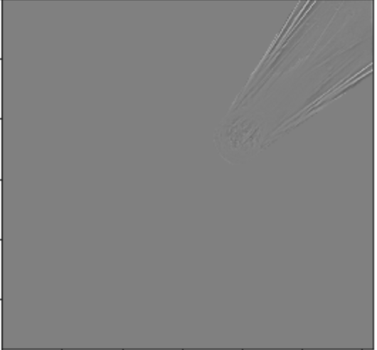
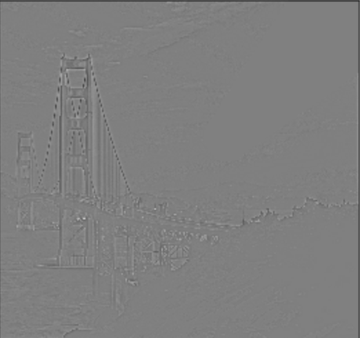
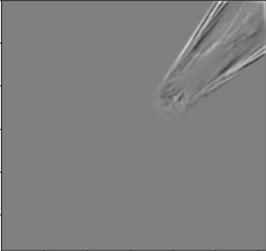
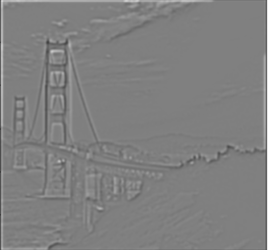
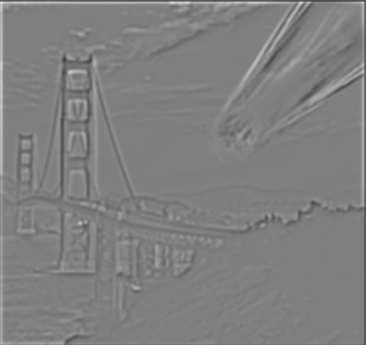
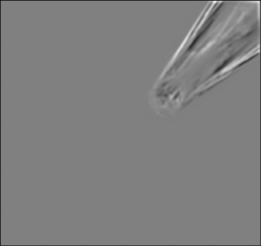
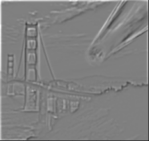
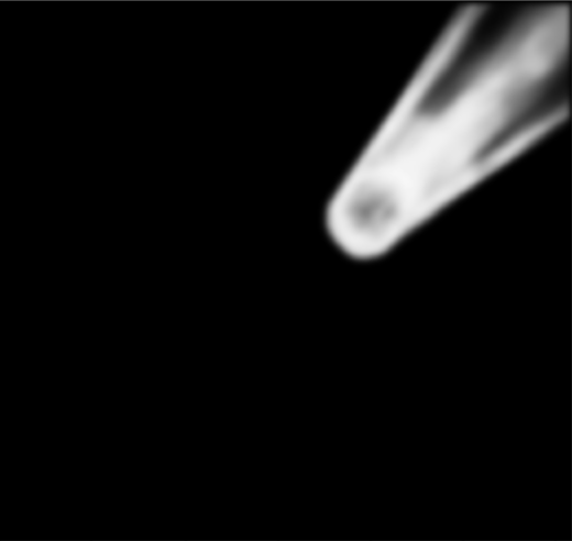
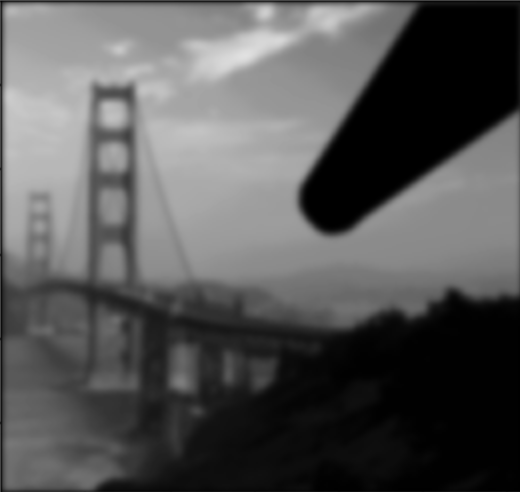
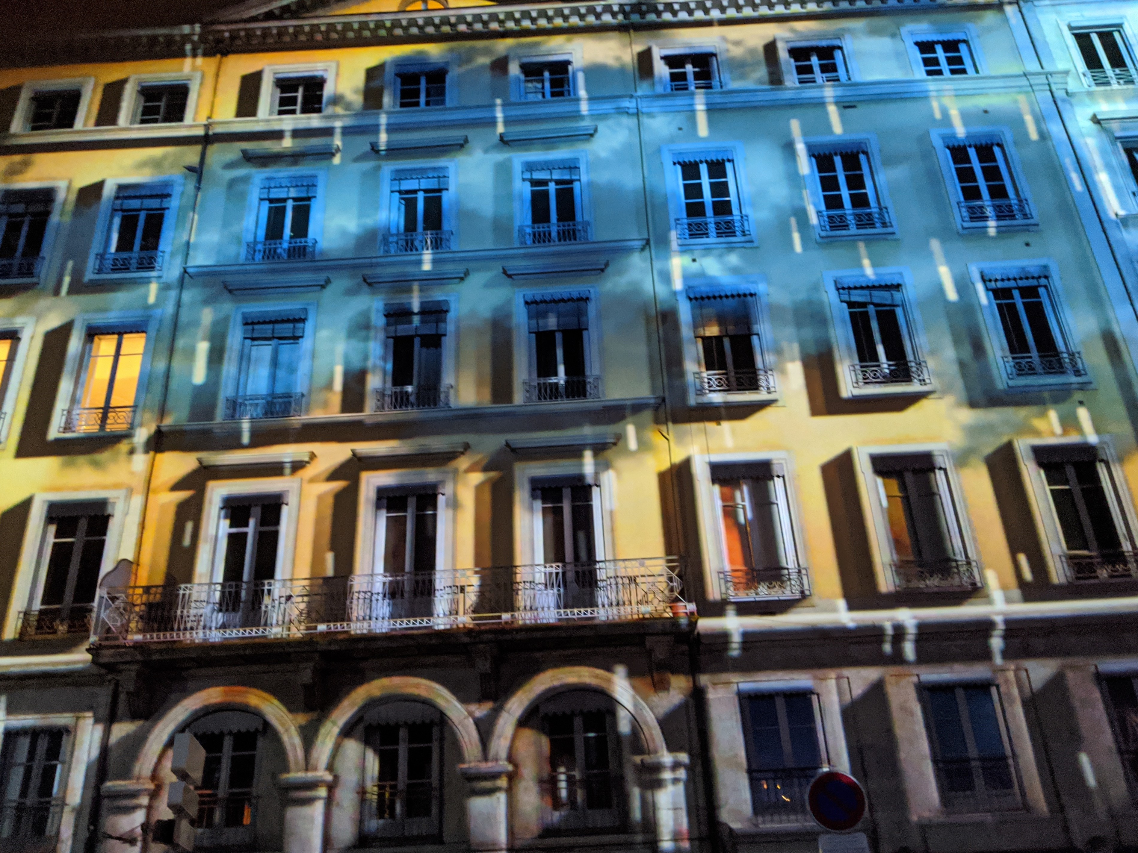
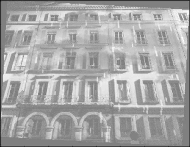
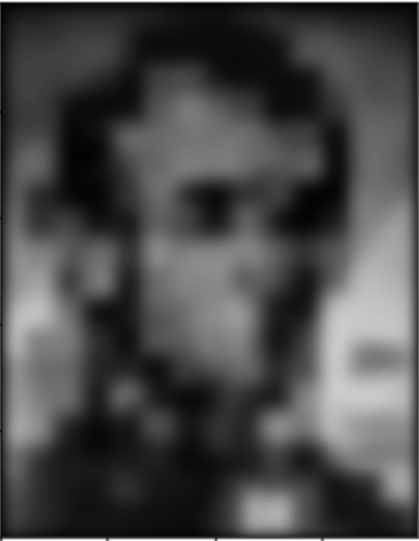
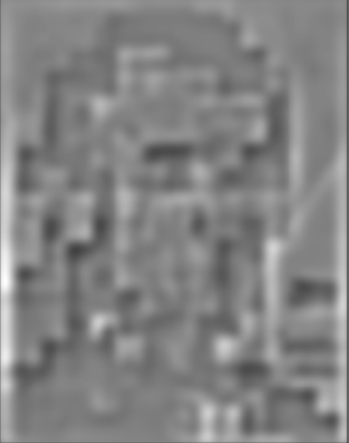
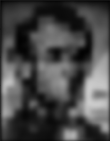
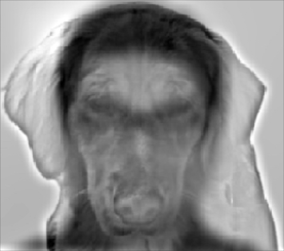
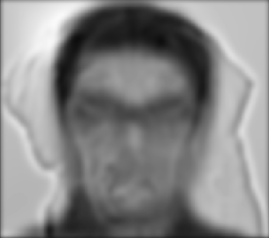
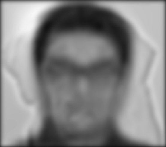
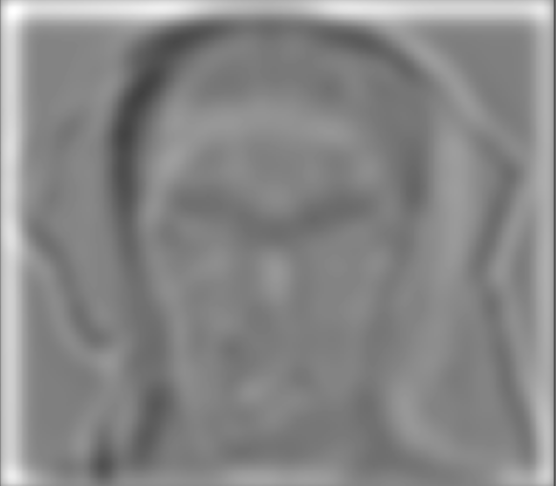
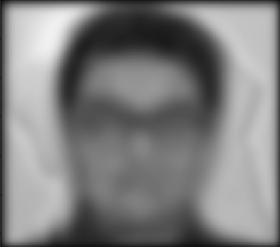
In this part, the goal was to make hybrid images. We combined 2 images to form a hybrid image where one could be seen from a certain distance and the other from further away. In order to achieve this effect, I extracted the high frequencies of one of the images and the low frequencies of the other and then superimposed them to create the hybrid image.

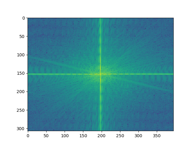
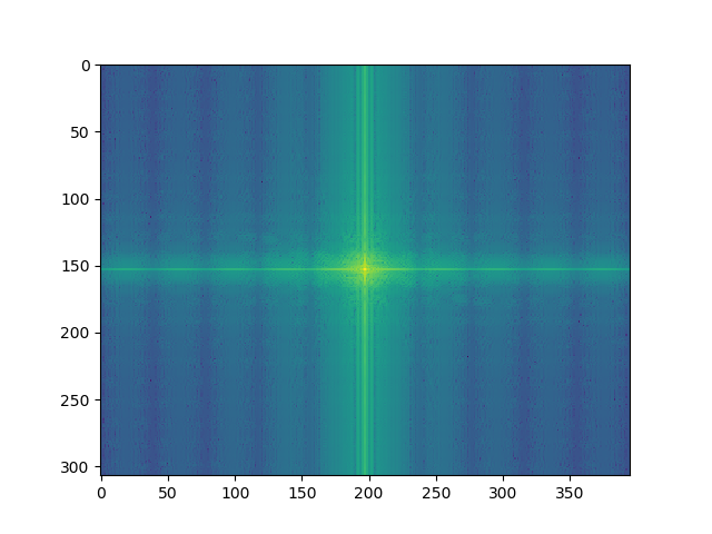
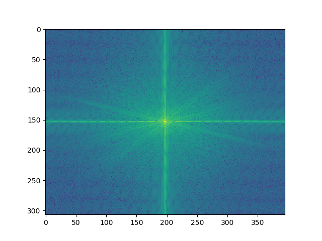

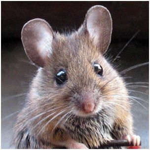
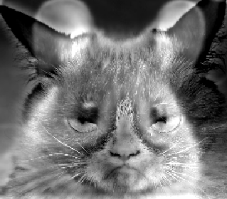
Hybrid Images only look appropriate when the 2 images have shapes that can align and match up. This is why faces work well. However objects that have different shapes do not align well when superimposed.


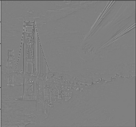
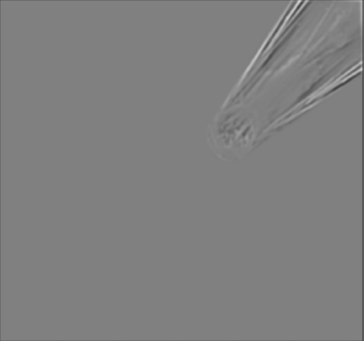
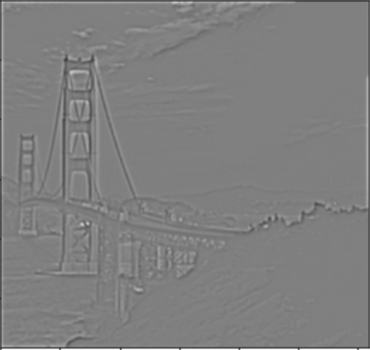
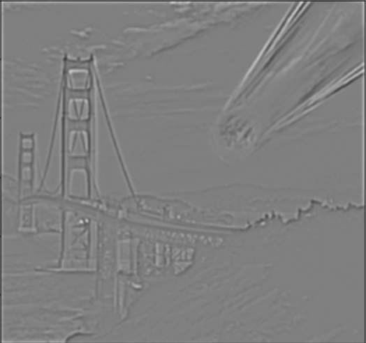
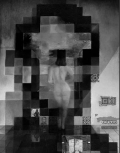
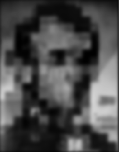
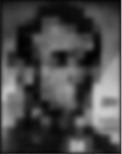
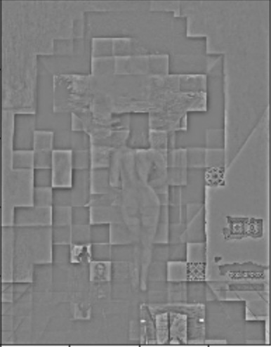
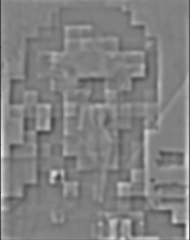
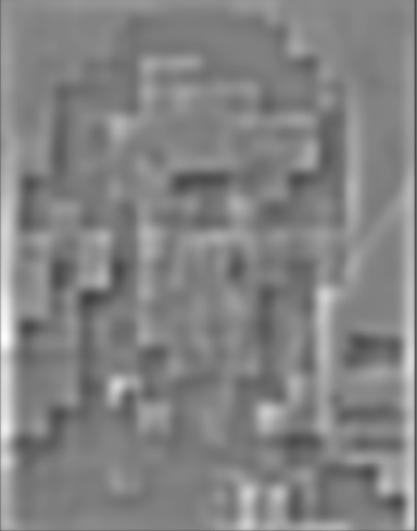
For this part, we had to generate the LaPlacian and Guassian stacks for 2 hybrid style images.


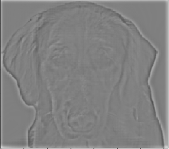
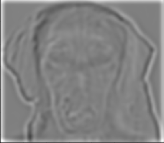
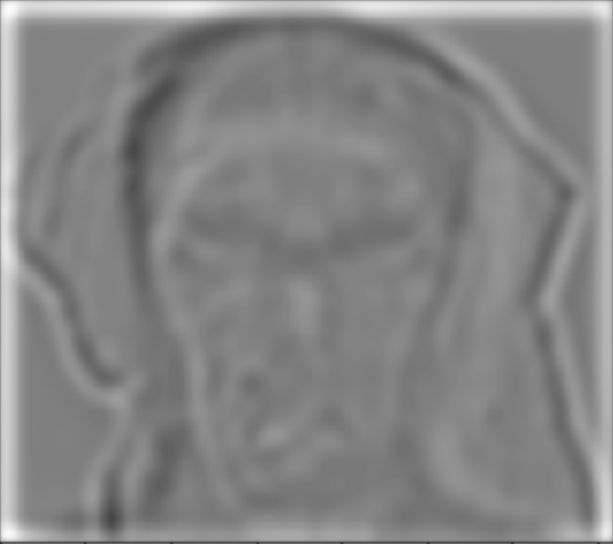
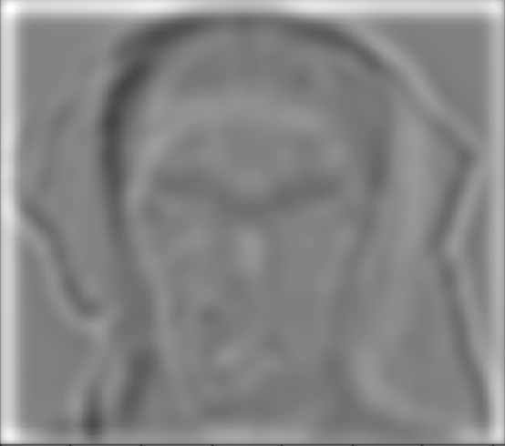
I performed image blending of 2 different images using a provided mask.