partial derivative w.r.t. x
partial derivative w.r.t. x
partial derivative w.r.t. y
gradient magnitude
binarized gradient magnitude (.15)
partial derivative w.r.t. x
partial derivative w.r.t. y
gradient magnitude
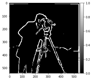
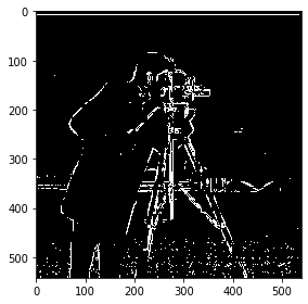
binary gradient magnitude (.05)
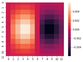
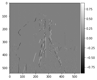
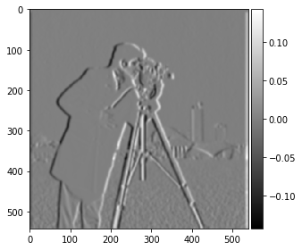
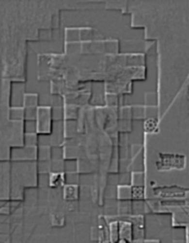
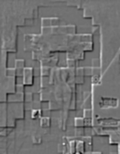
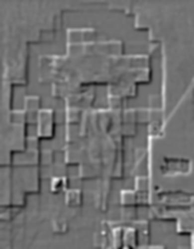
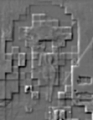
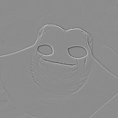
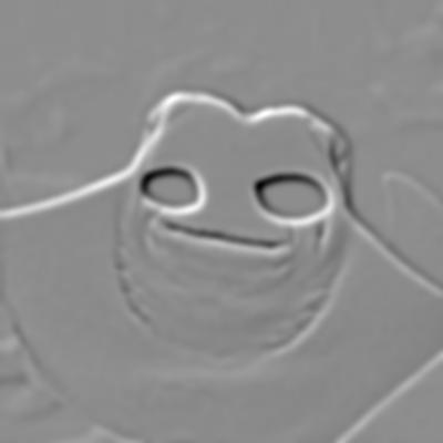
partial derivative of gaussian w.r.t. x
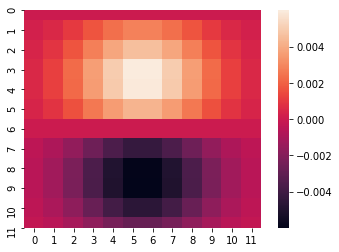
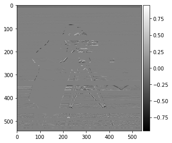
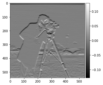
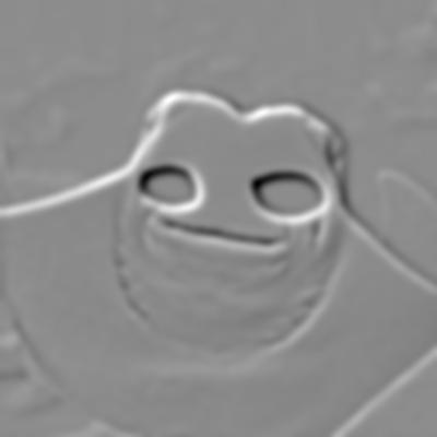
partial derivative of gaussian w.r.t. y
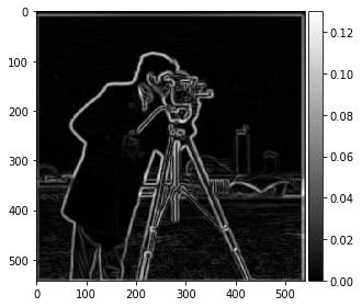
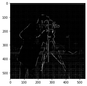
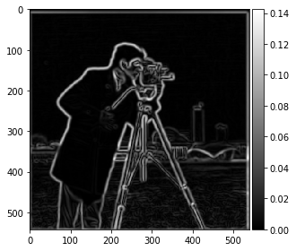
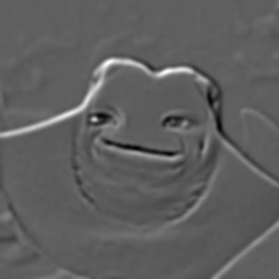
gradient magnitude using derivatives of gaussian
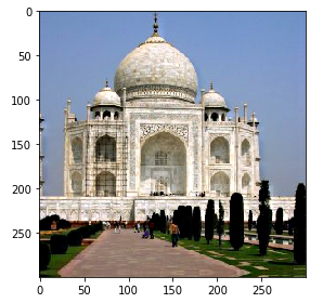
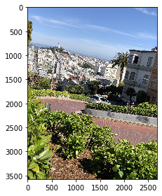
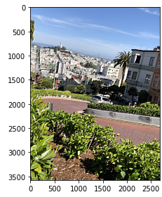
original
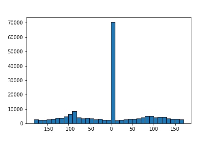
original angle histogram
straightened
straightened angle histogram
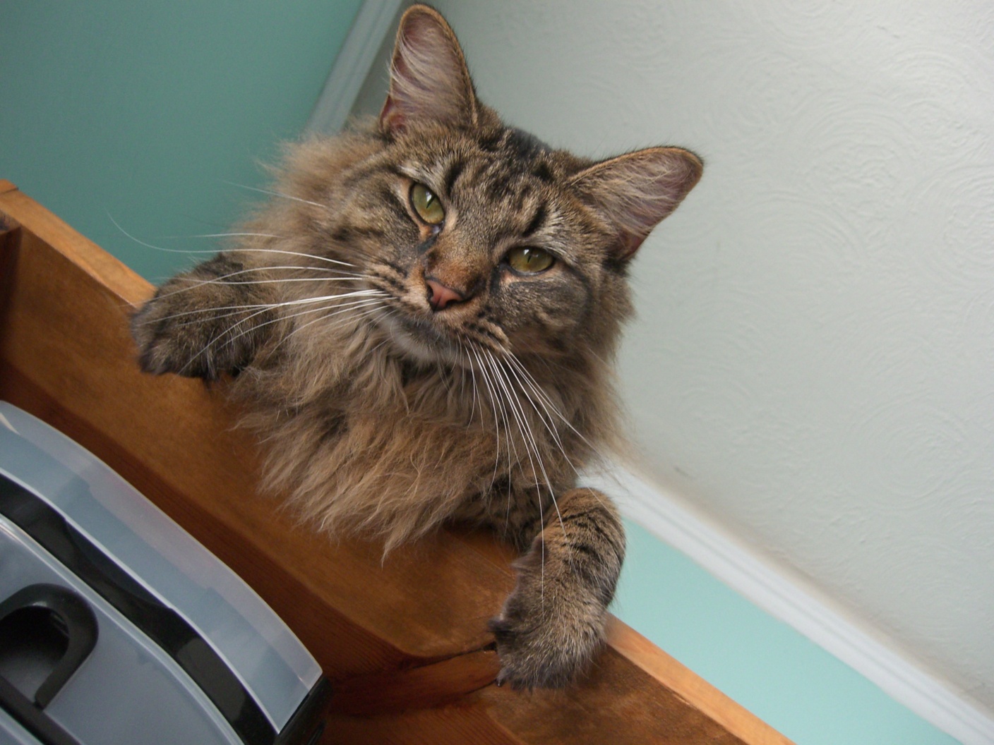
original
original angle histogram
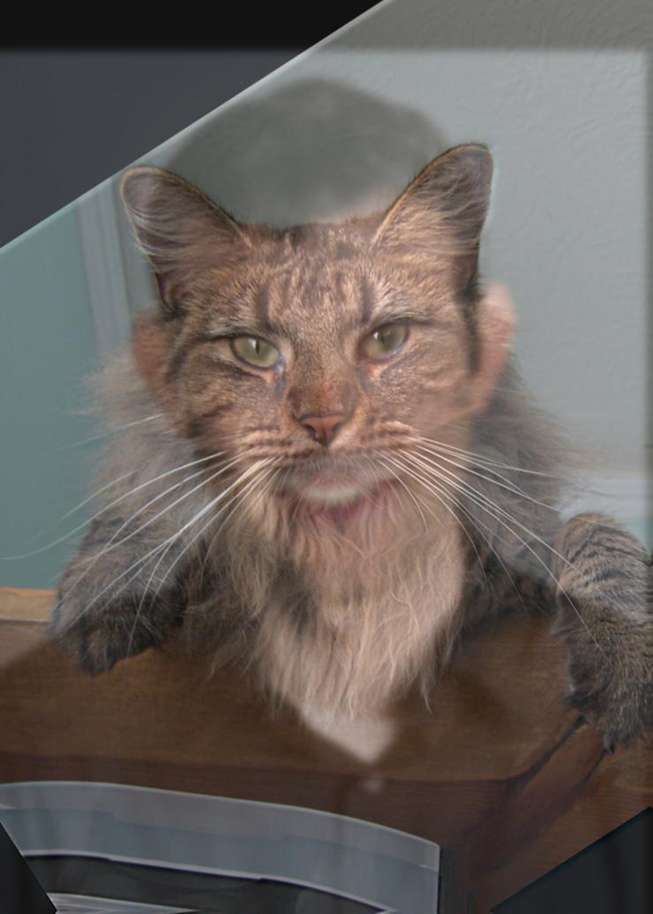
straightened
straightened angle histogram

original
original angle histogram
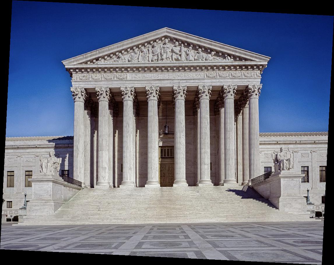
straightened
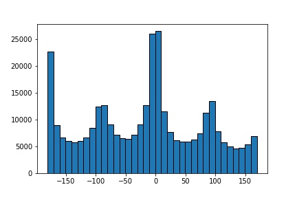
straightened angle histogram
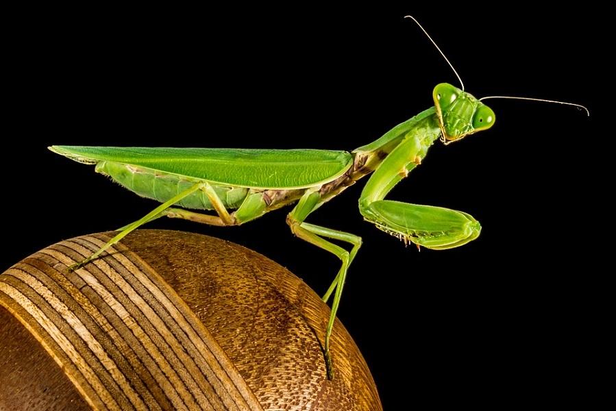
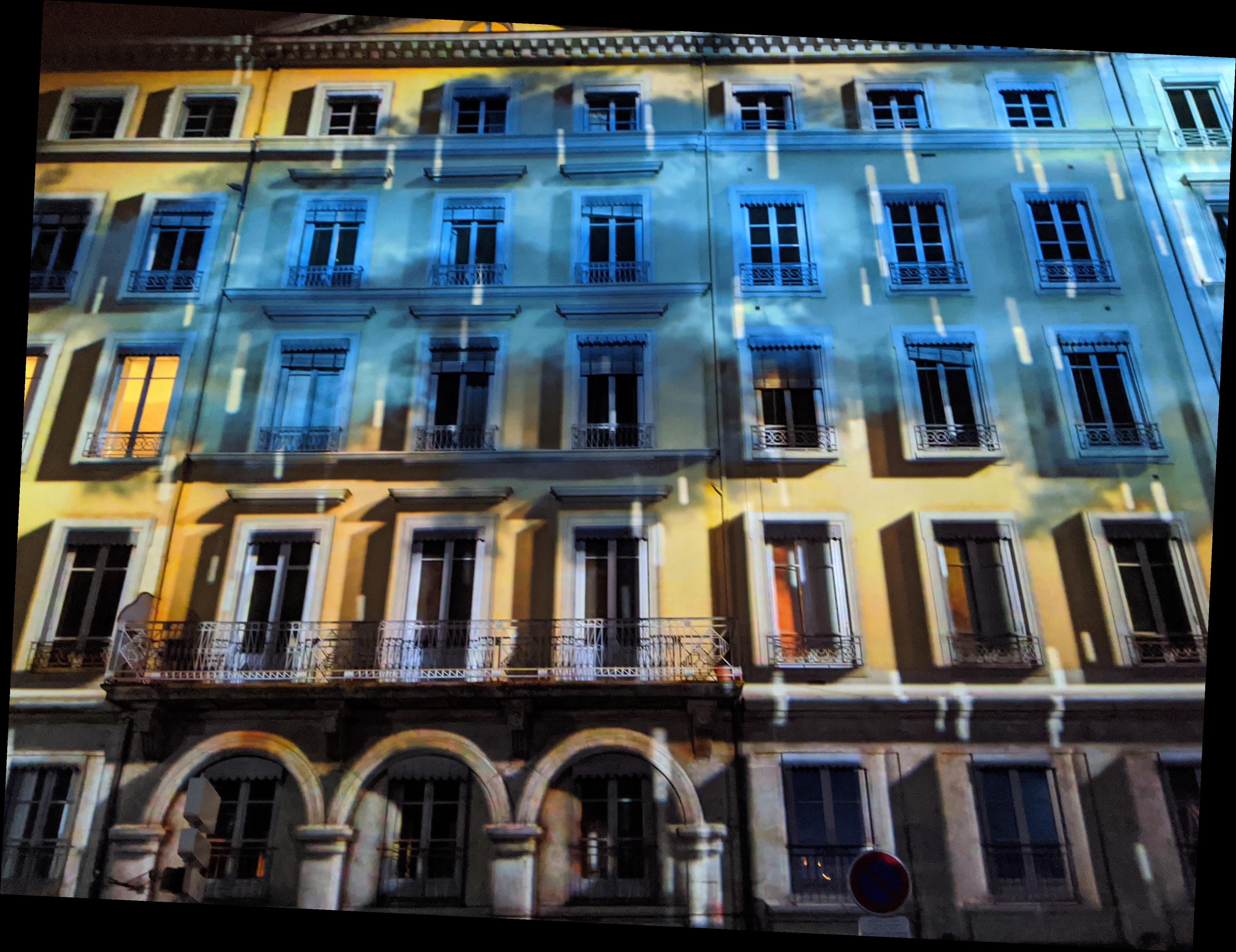
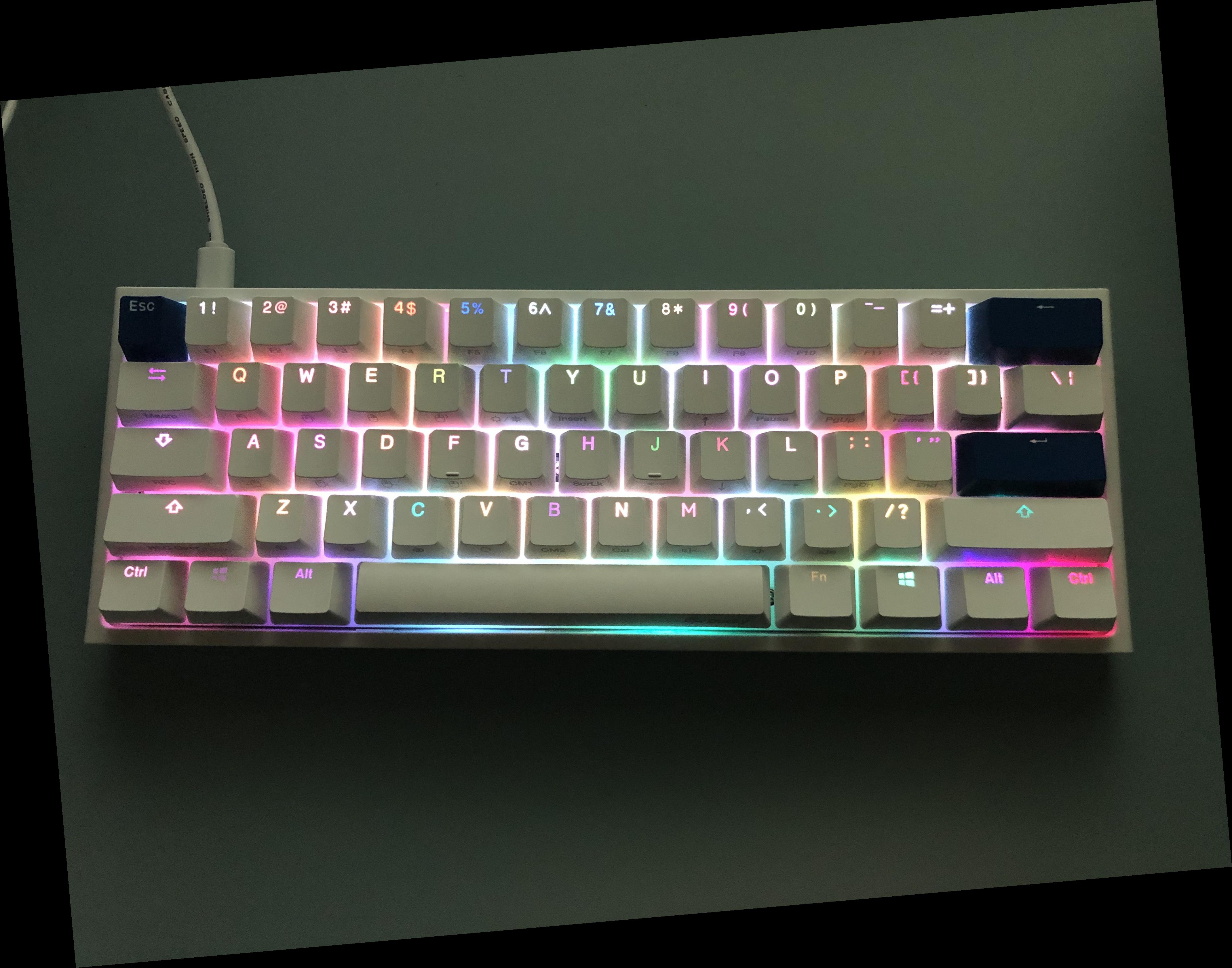
original
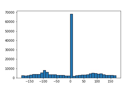
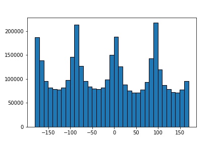
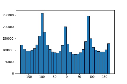
original angle histogram
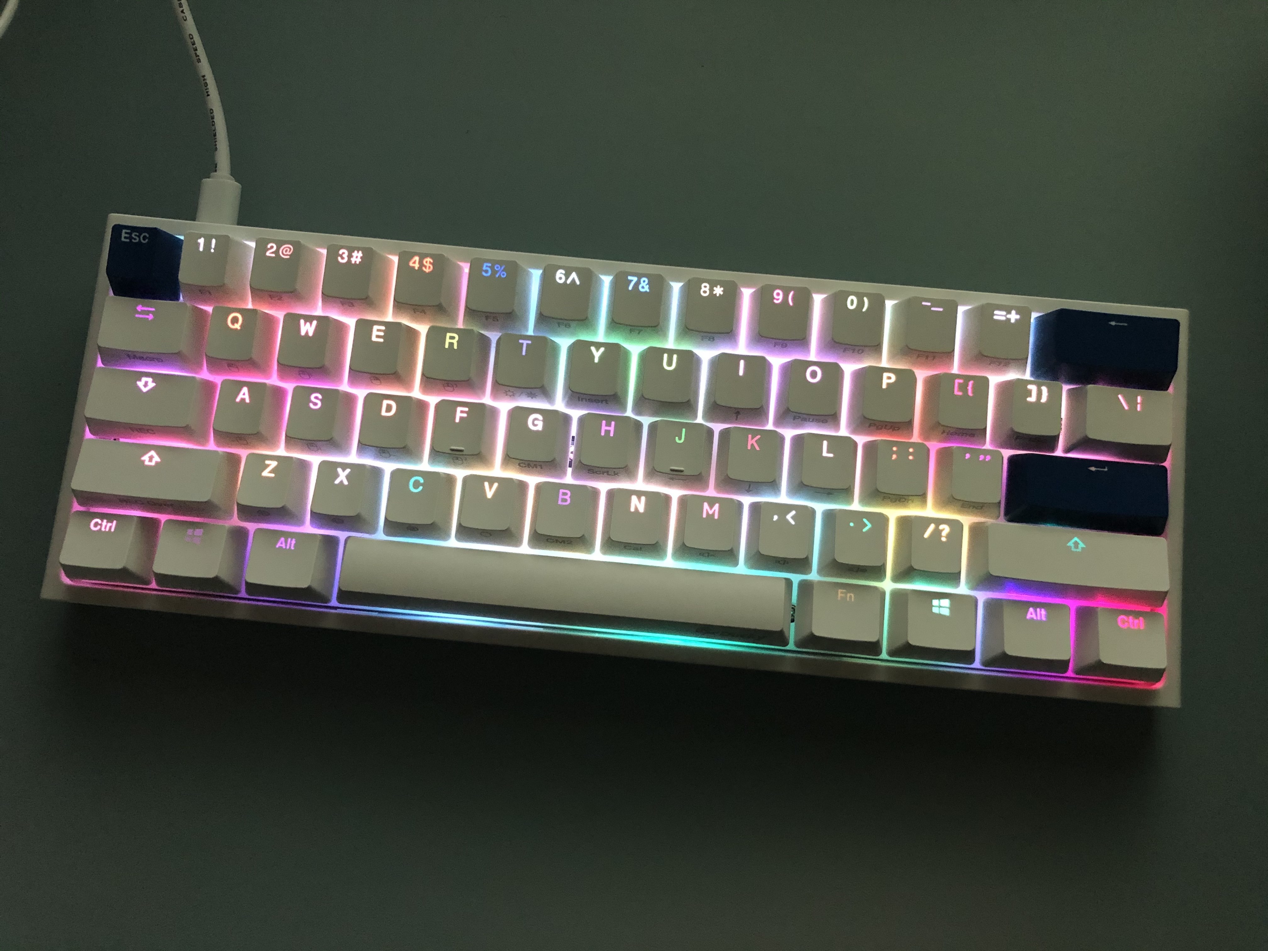
"straightened"
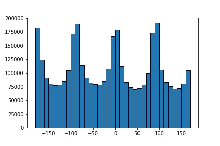
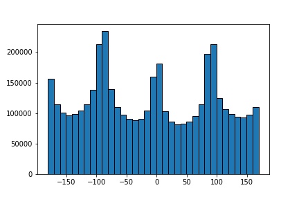
straightened angle histogram

original
sharpened
original

blurred
resharpened
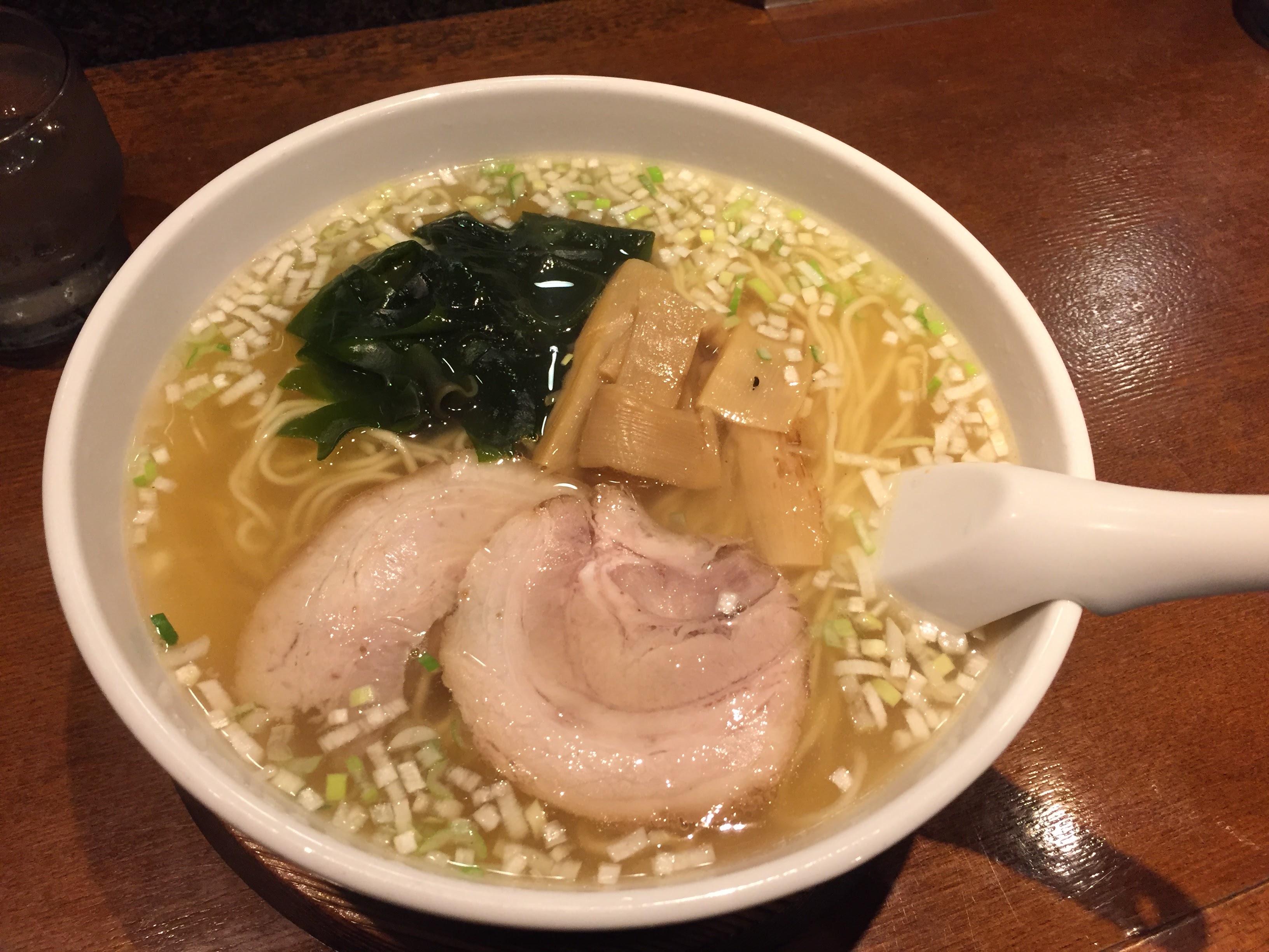
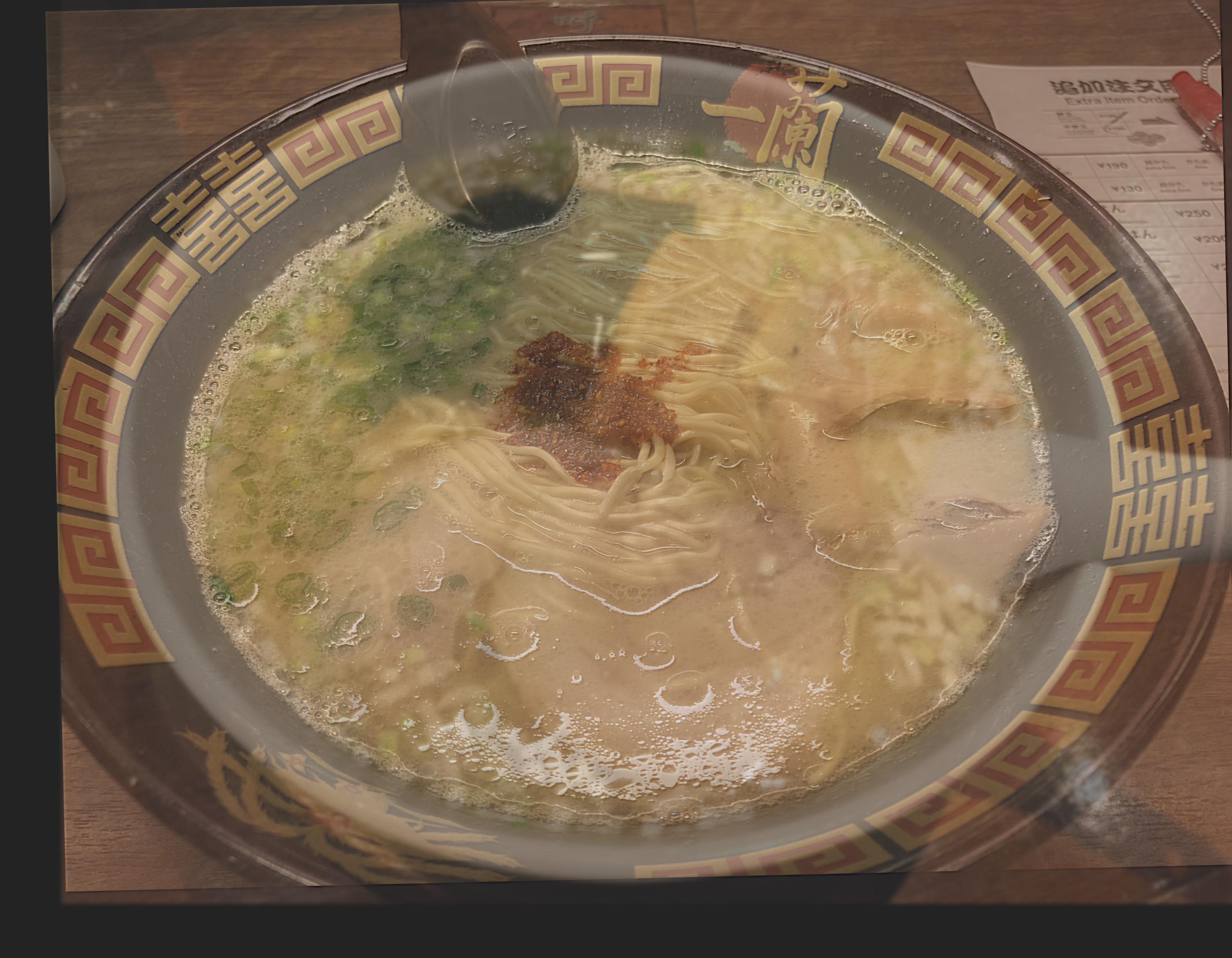
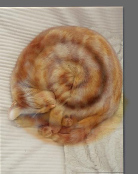
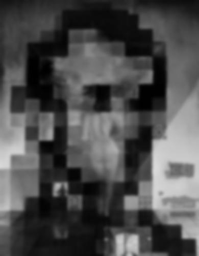
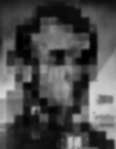
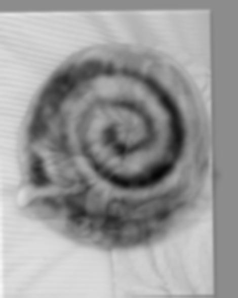
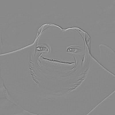
high freq input

low freq input
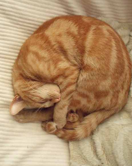
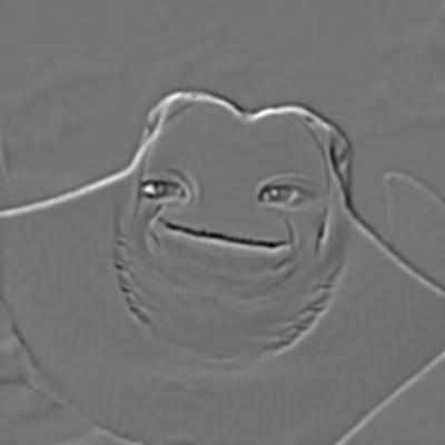
hybrid result
high freq input
low freq input
hybrid result
high freq input
low freq input
hybrid result
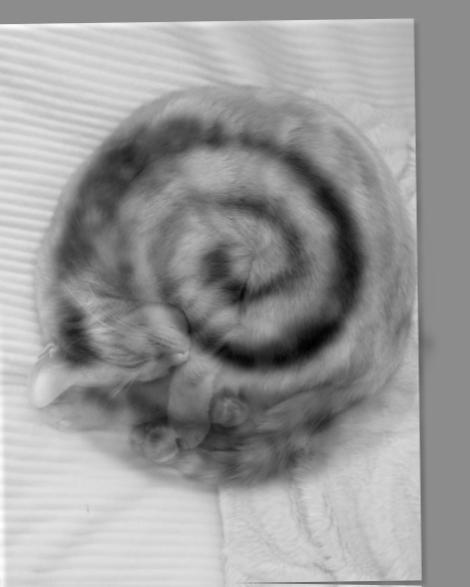
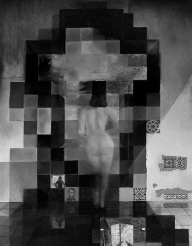
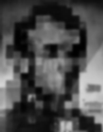
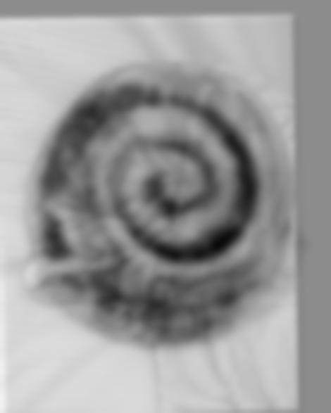
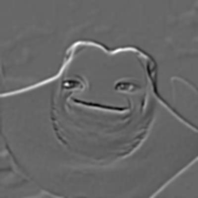
gray hybrid result
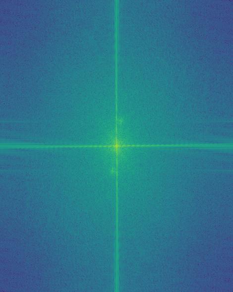
high freq input FT
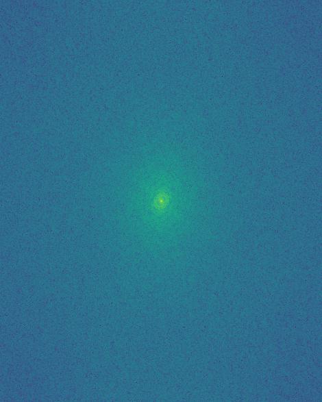
low freq input FT
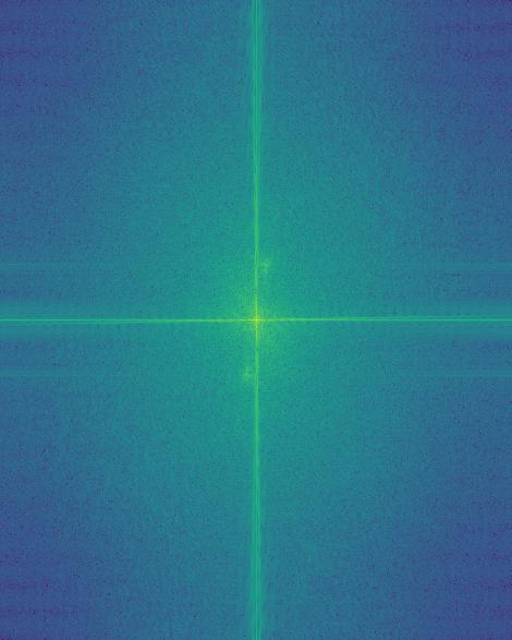
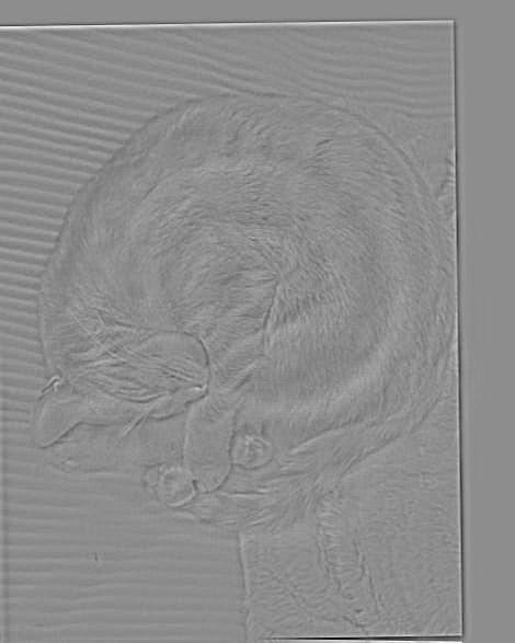
high pass filtered FT
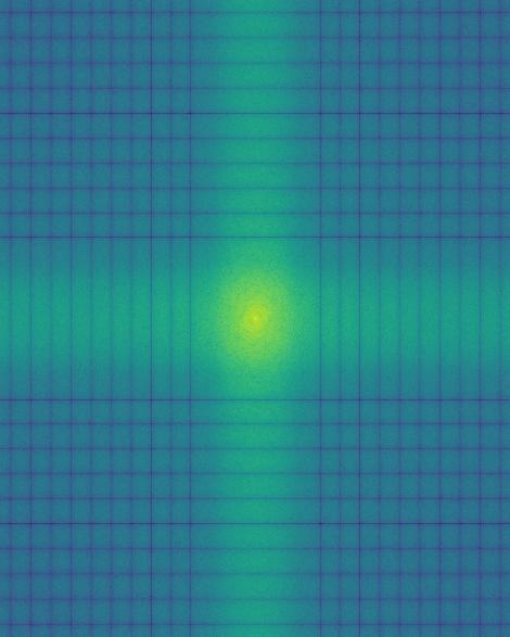
low pass filtered FT
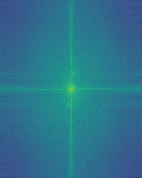
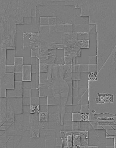
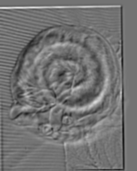
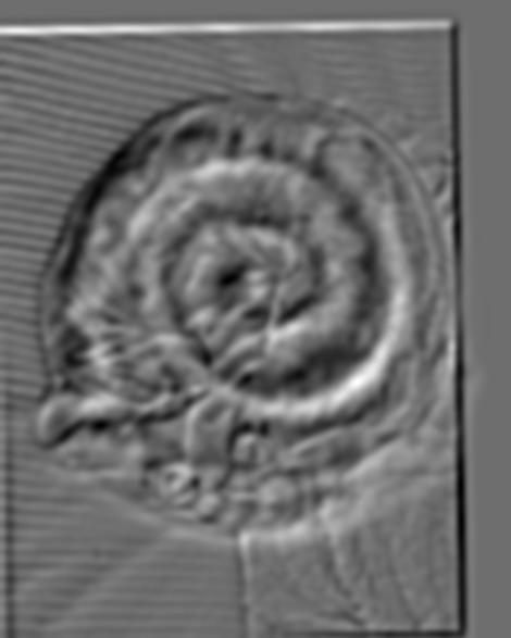
gray hybrid result FT
|

|
|

|
|
|
|
|
|
|
|

|

|

|
|

|

|
|
|

|
|

|
|

|

apple

orange

mask

blended
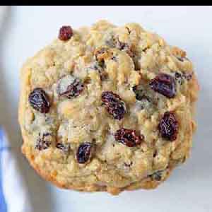
oatmeal raisin cookie
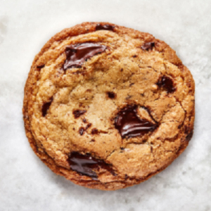
chocolate chip cookie
mask
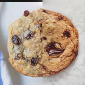
blended
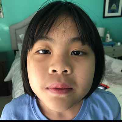
human

stingray

mask

blended
|
|
|
|

|

|
|

|

|
|
|

|

|

|
|
|
|

|