Fun with Filters and Frequencies!

CS 194-26 Project 2 Fall 2020

Glenn Wysen

lincoln
Fig.1 - A Dali painting of Abe Lincoln and and a woman that changes based on frequency.

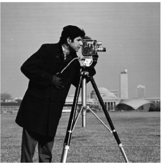
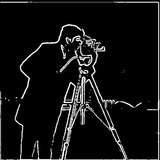
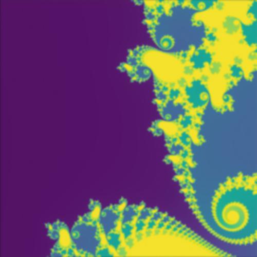
Gradient Magnitude Image

The gradient magnitude image is calculated by running a horizontal edge gradient filter and a vertical edge gradient filter over the image and then combining the results. First, a Gaussian blur is applied across the original image to reduce gradient detection of noise in the image. Next, the horizontal and vertical gradient magnitude images are calculated by convolving a simple difference filter over the blurred image. Finally, the two gradient images are added together, normalized, and binarized to 0 or 1 based on an arbitrary threshold (I used 0.3).

doorway
Fig.2 - Original cameraman image.
doorway
Fig.3 - Horizontal edges detected.
doorway
Fig.4 - Vertical edges detected.
cameraman
Fig.5 - Combined horizontal and vertical images and rescaled to black and white.

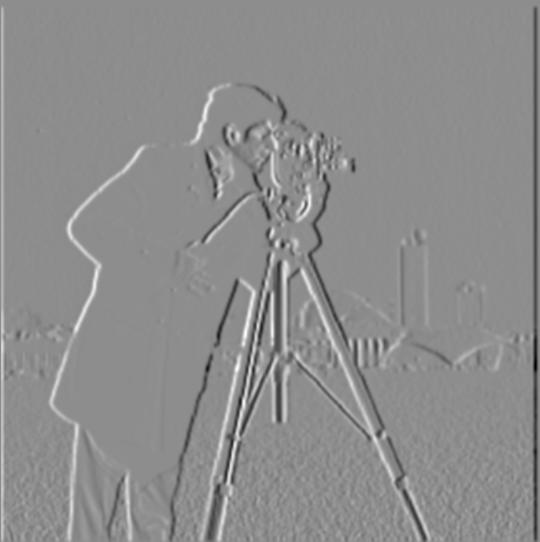
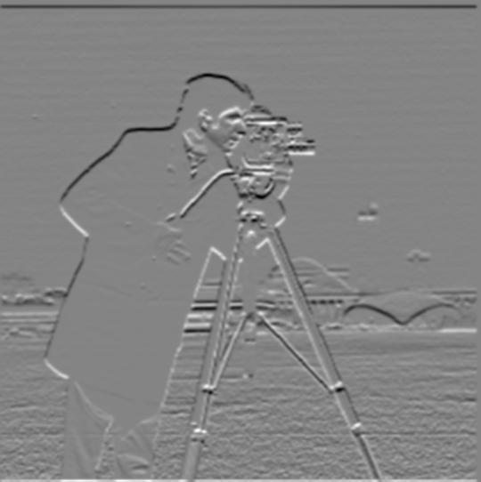
Derivative of Gaussian (DoG) Filter

By adding a Gaussian blur, the horizontal and vertical derivative filters became less affected by random noise in the image. This meant that the filtered images became much smoother. When I convolved the D_x and D_y filters with the Gaussian blur and then convolved the resulting filter with the original image I got the same result as doing all three separately.

Image Straightening

Image straightening was implemented by convolving the image with the horizontal and vertical derivative filters and then calculating the angle of the gradient at each point. After this, the image was rotated through a -20 to +20 degree range from vertical. In each step the number of points with a gradient within 5 degrees of horizontal and vertical were calculated and the rotation with the highest number of these points was selected as the straightened image.
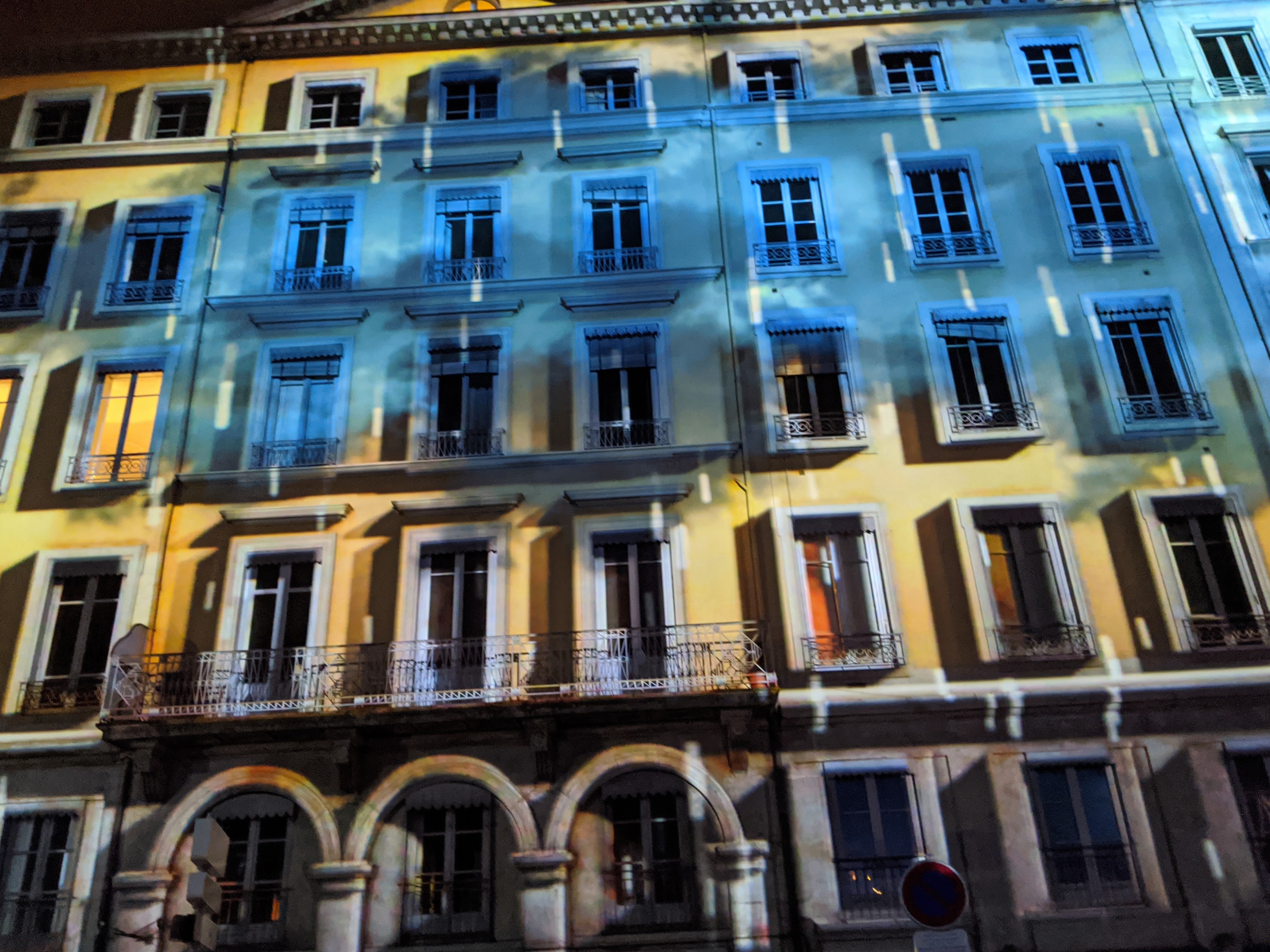
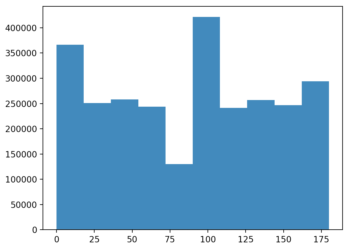
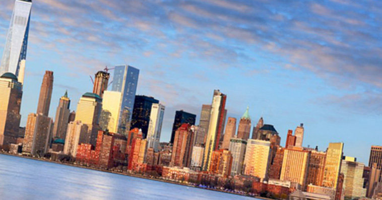
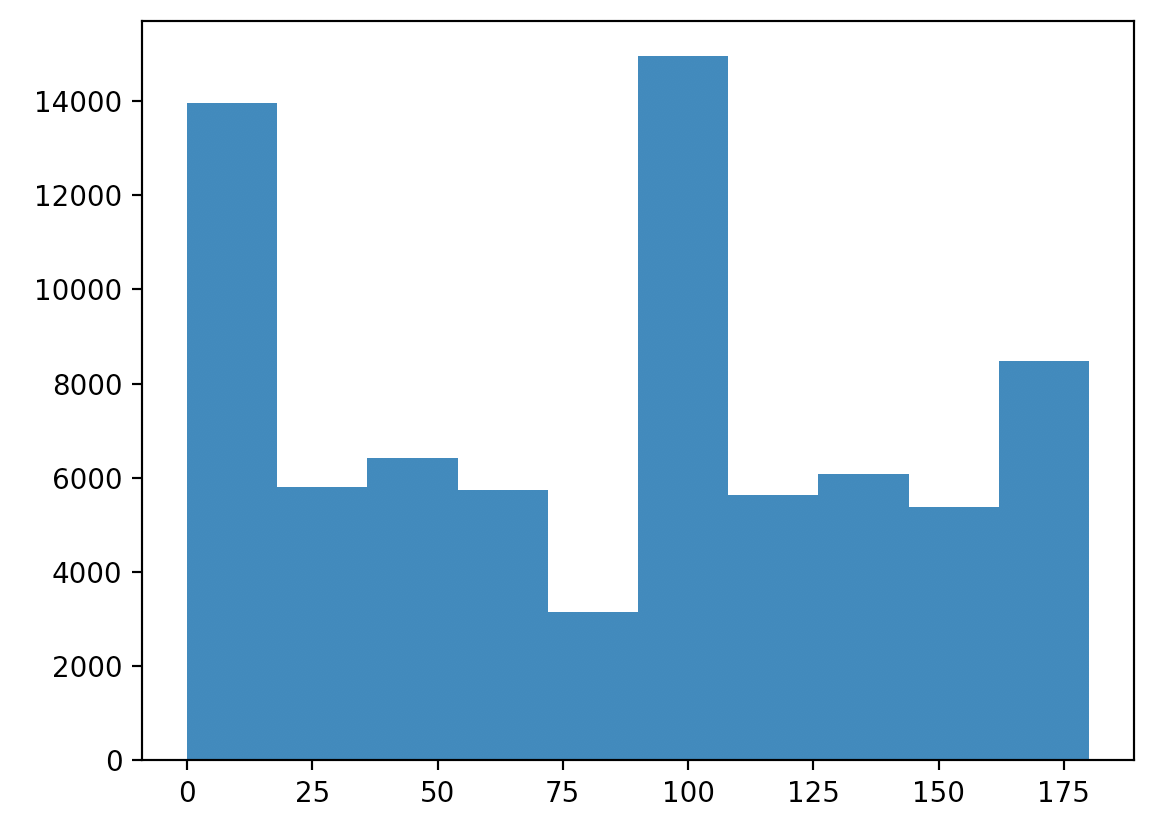
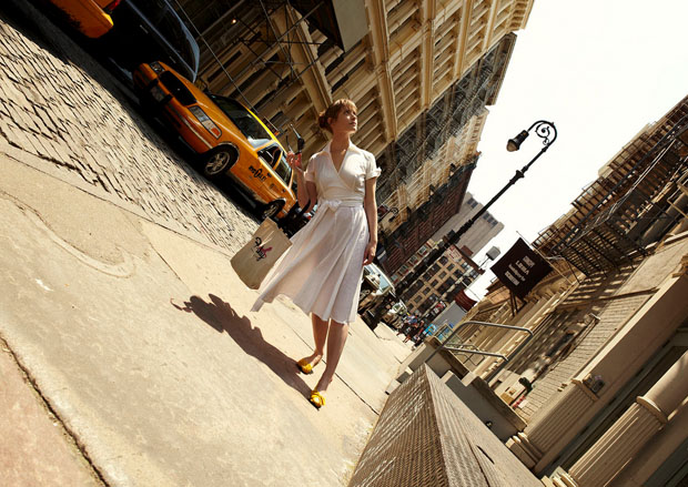
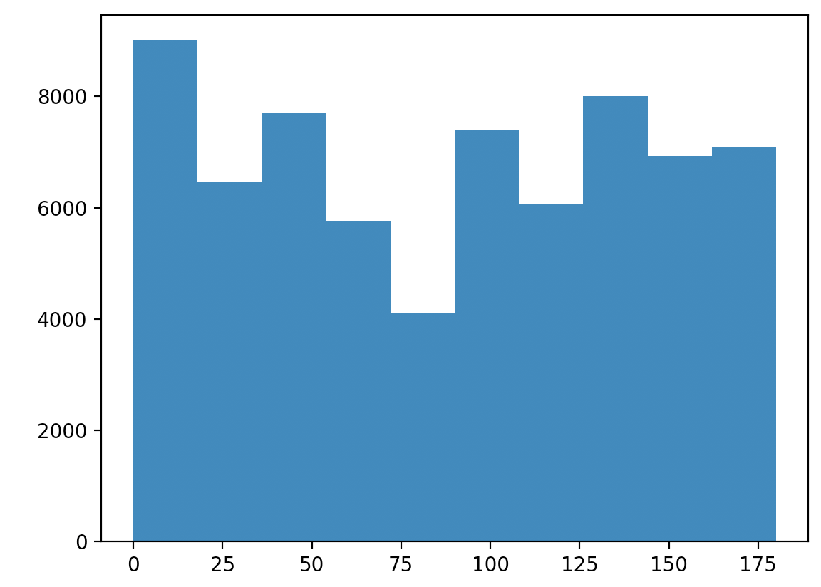
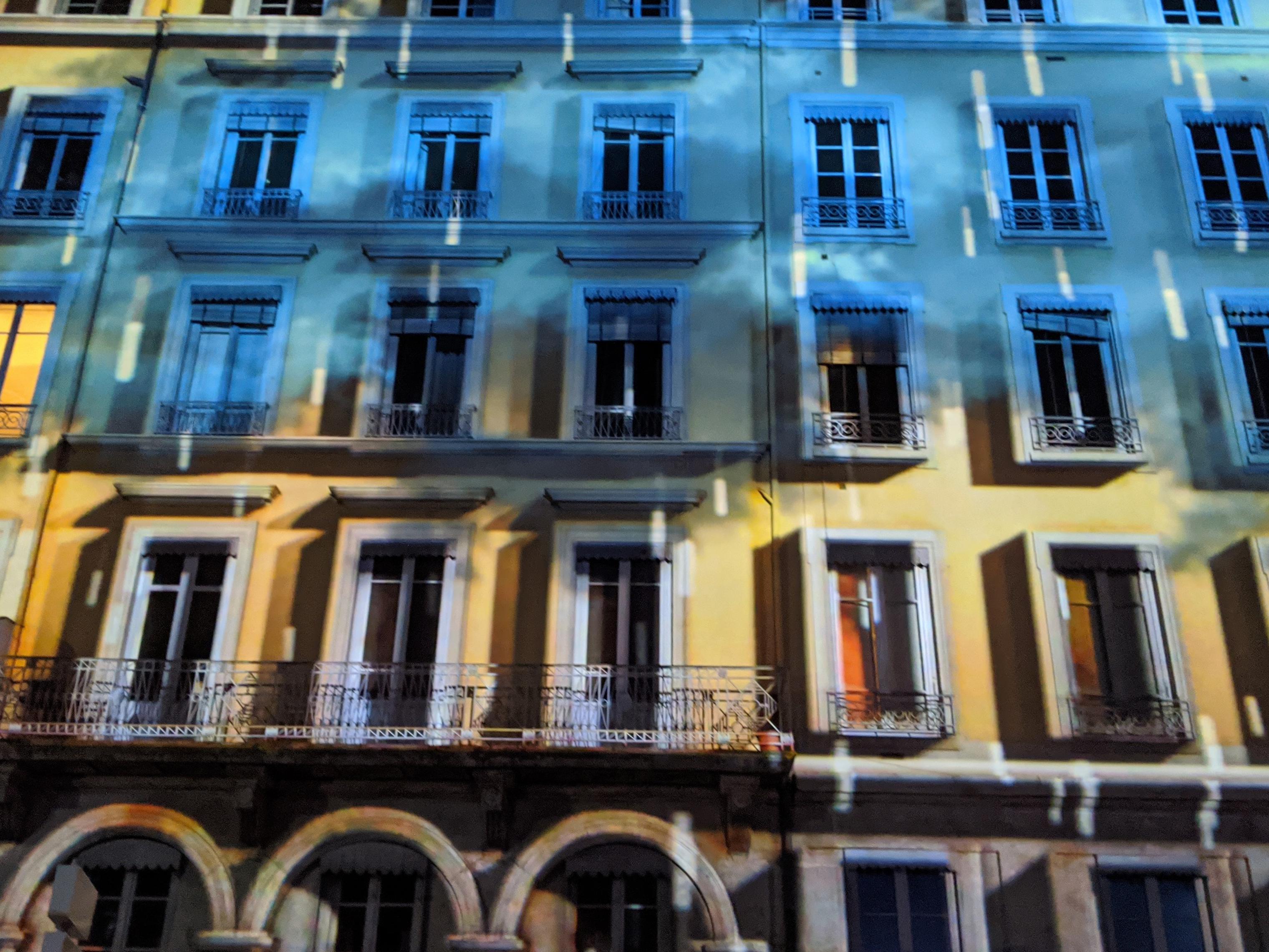
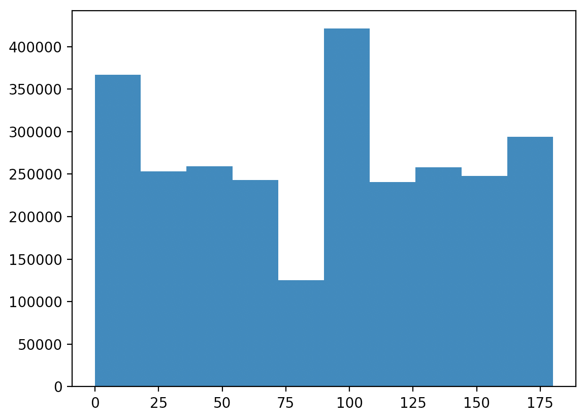
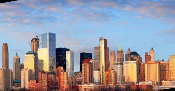
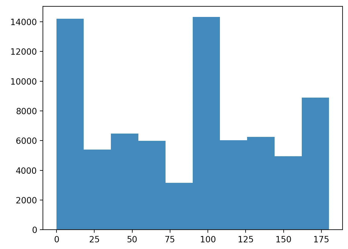
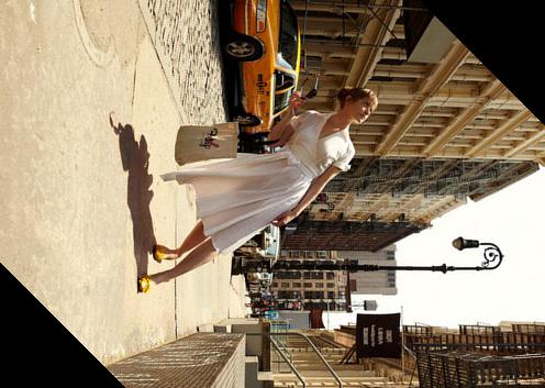
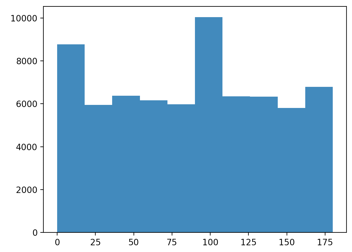
doorway
Fig.6 - Original facade image.
doorway
Fig.7 - Original facade histogram.
doorway
Fig.10 - Original skyline image.
doorway
Fig.11 - Original skyline histogram.
doorway
Fig.14 - Original woman image.
doorway
Fig.15 - Original woman histogram.
doorway
Fig.8 - Straightened facade image.
cameraman
Fig.9 - Straightened facade historgram.
doorway
Fig.12 - Straightened skyline image.
cameraman
Fig.13 - Straightened skyline historgram.
doorway
Fig.16 - Straightened woman image that failed as the program thought sideways was vertical because there was no differentiation between horizontal and vertical orientations.
doorway
Fig.17 - Straightened woman histogram.

Image "Sharpening"

Image "sharpening" was implemented by taking an image, subtracting a Gaussian blur from the image, and then adding the subtraction back into the original image to highlight the high frequencies.
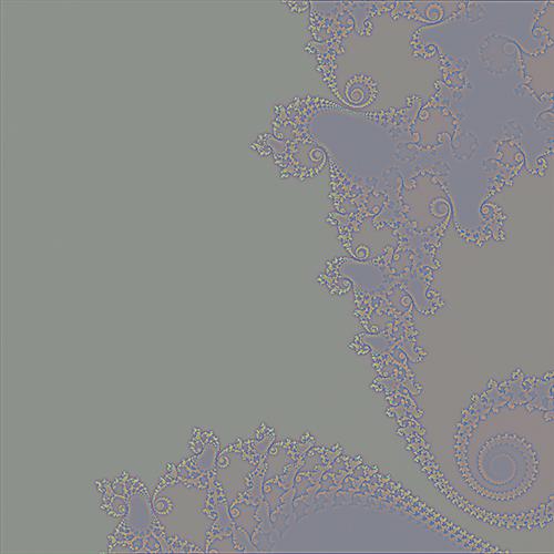
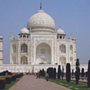
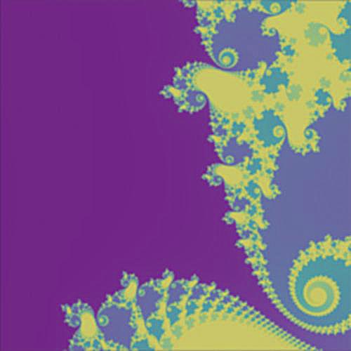
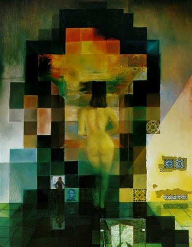
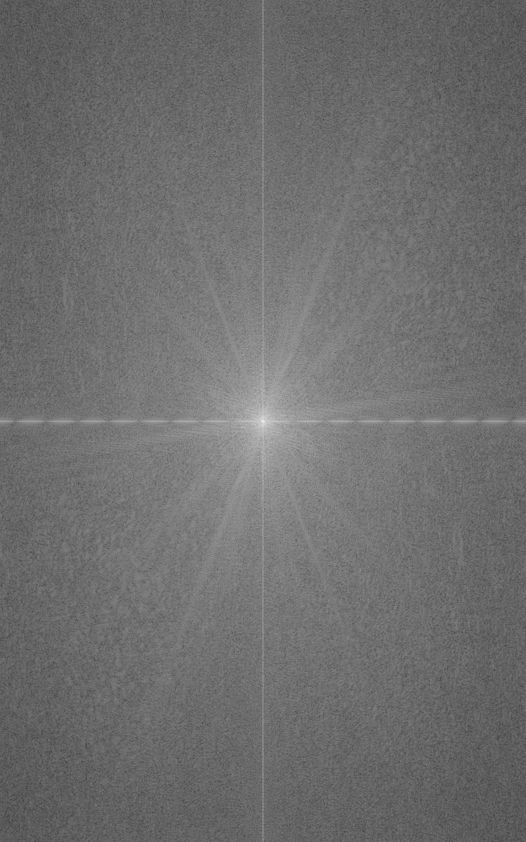
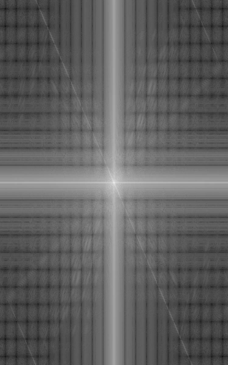
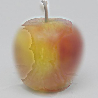
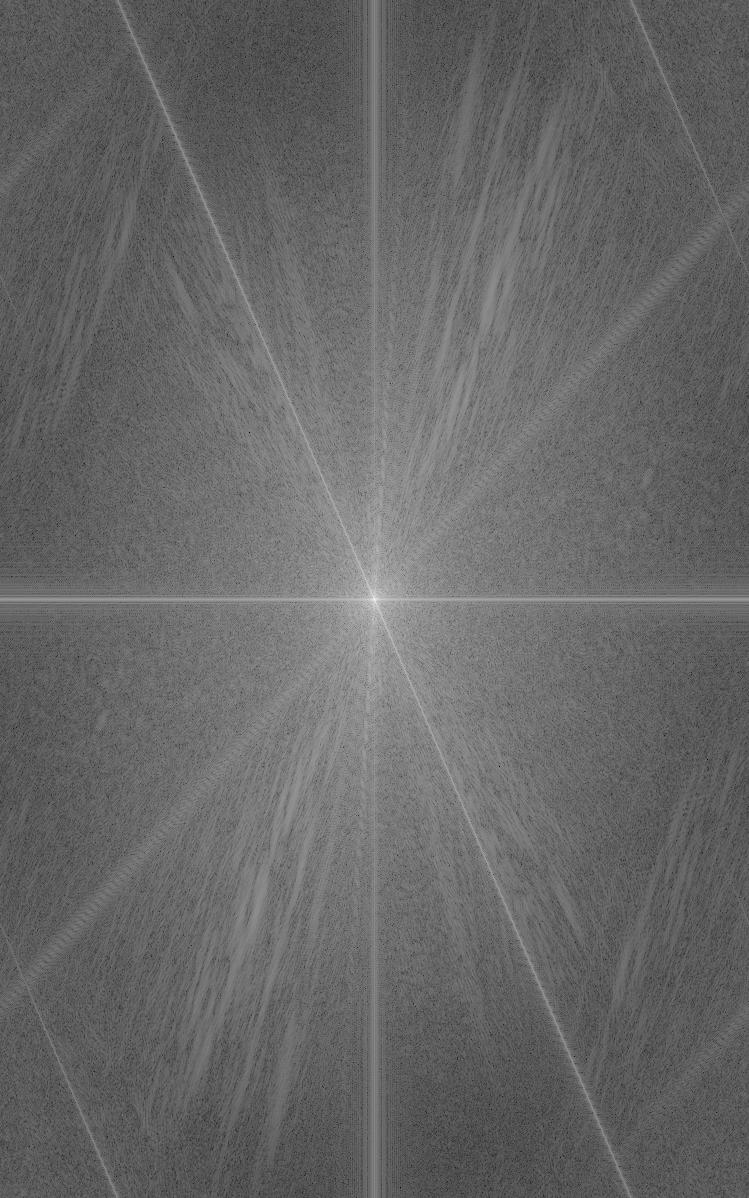
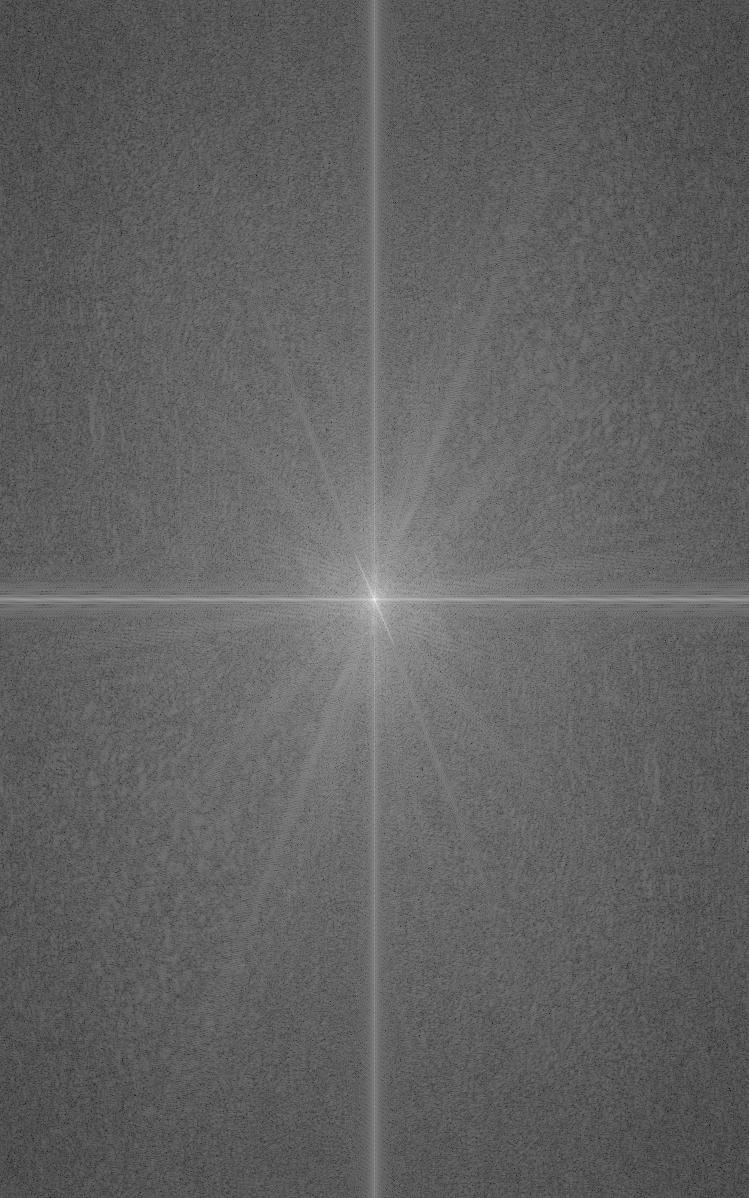
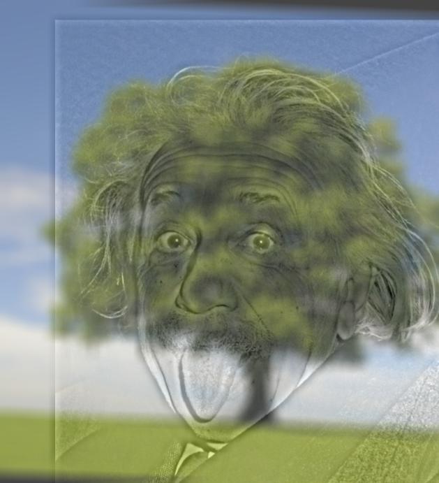
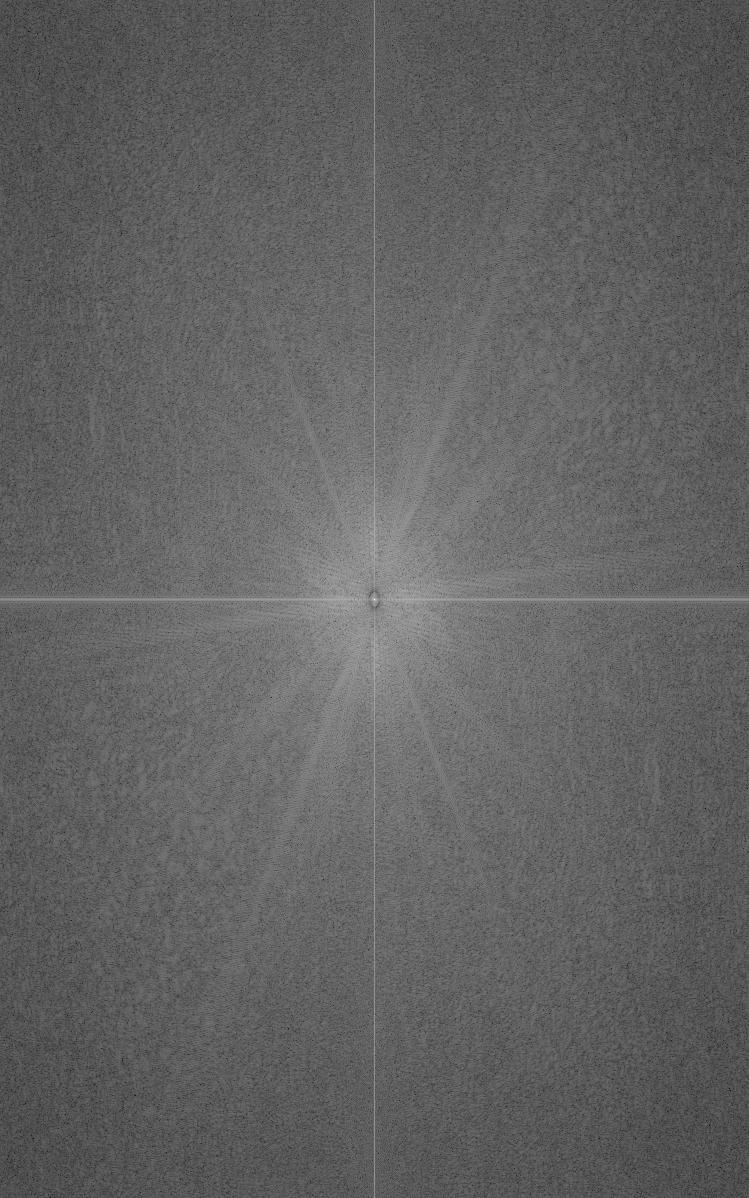
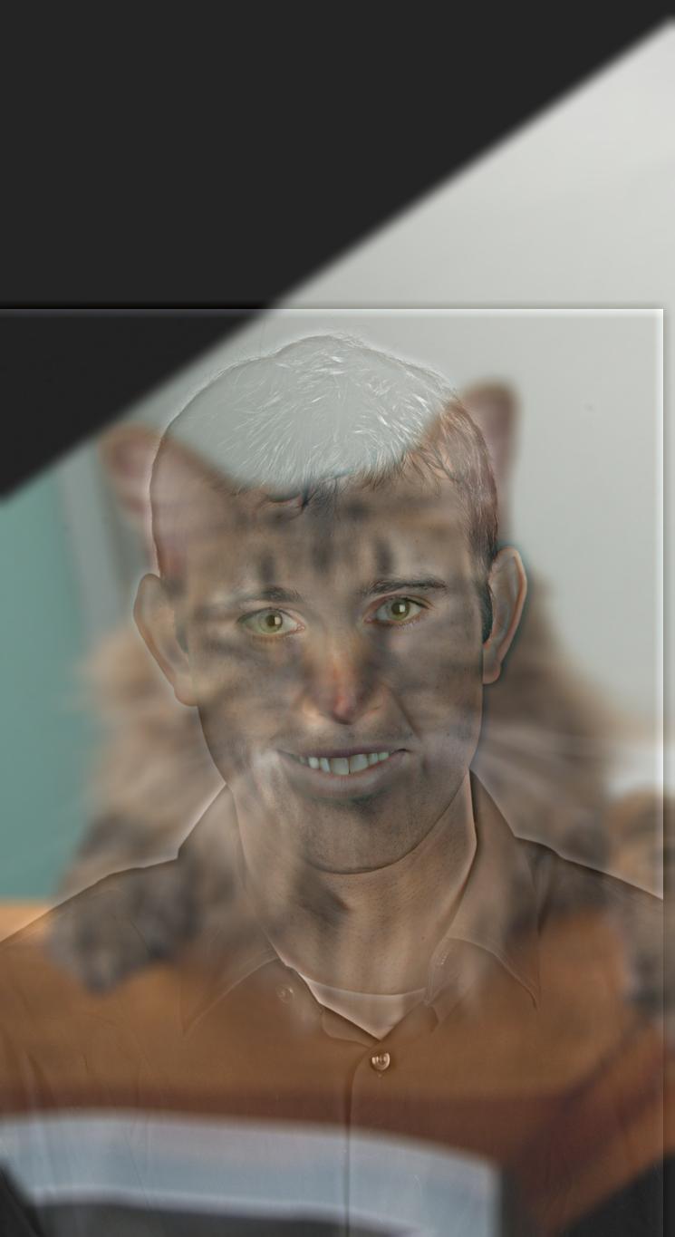
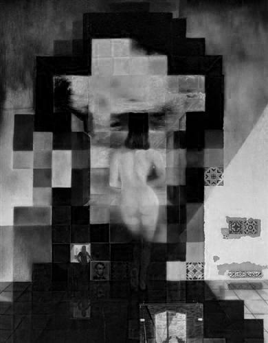
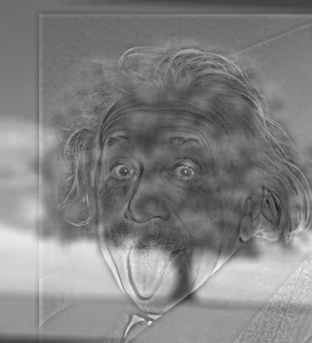
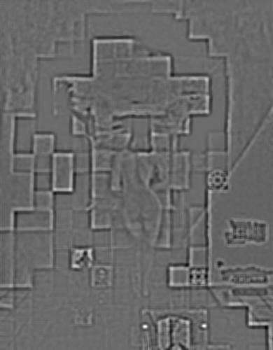
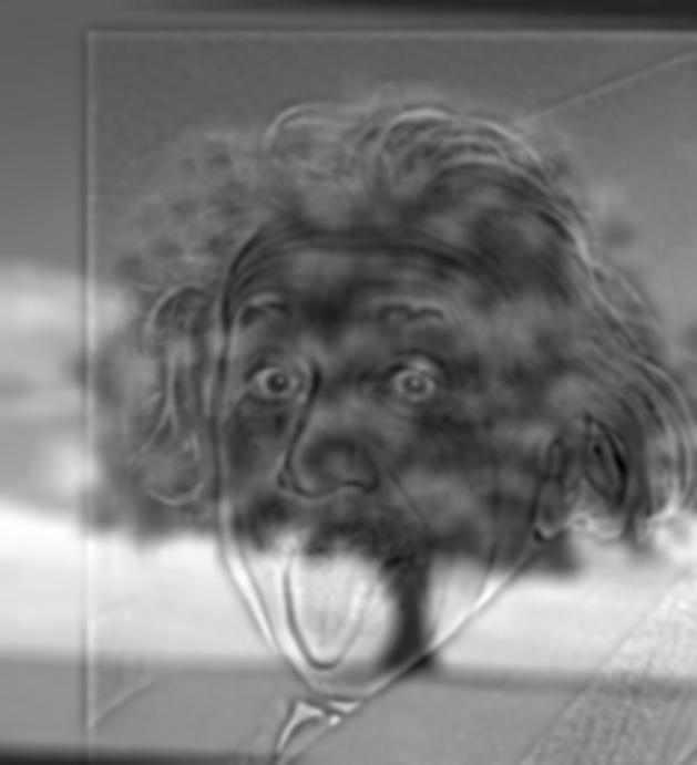
doorway
Fig.18 - Original blurry image.
doorway
Fig.21 - Original blurry image.
doorway
Fig.19 - High frequency mask.
doorway
Fig.22 - High frequency mask.
doorway
Fig.20 - Resulting "sharper" image.
doorway
Fig.23 - Resulting "sharper" image.

Hybrid Images

Hybrid images were created by taking the high frequencies of one image (obtained by subtracting the Gaussian blur of an image from the original) and combining it with the low frequencies of another image. The resulting image will look one way from close up and another way from far away based on the frequencies in the image.

doorway
Fig.24 - Frequencies of original Derek image.
cameraman
Fig.27 - Frequencies of lowpass filtered nutmeg the cat.
cameraman
Fig.30 - Hybrid image of an apple and it's core.
doorway
Fig.25 - Frequencies of original nutmeg the cat image.
doorway
Fig.28 - Frequencies of final hybrid image.
cameraman
Fig.31 - Hybrid image of Einstein and a tree.
doorway
Fig.26 - Frequenices of highpass filtered Derek.
doorway
Fig.29 - Resulting hybrid image.

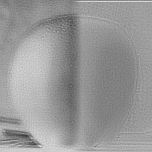
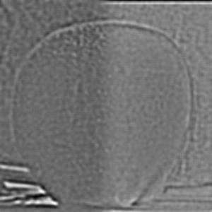
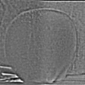
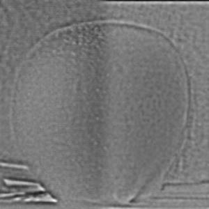
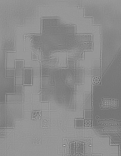
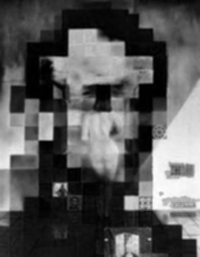
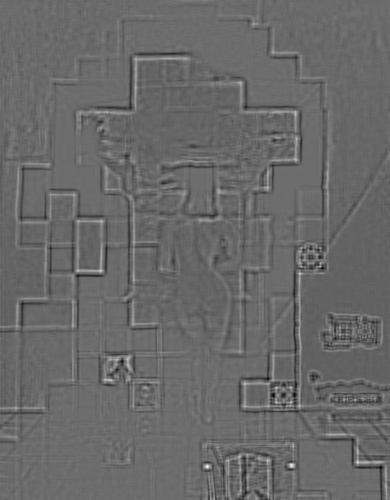
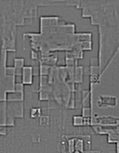
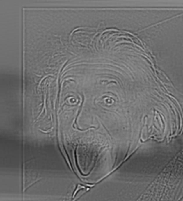
Gaussian and Laplacian Stacks

Gaussian and Laplacian stack are a way of storing different amounts of Gaussian blurring or Laplacian sharpening. Each layer of the Laplacian stack contained a further subtracted Gaussian to obtain a higher and higher frequency image.

doorway
Fig.31 - Level 1 of the Gaussian stack.
doorway
Fig.35 - Level 1 of the Laplacian stack.
doorway
Fig.39 - Level 1 of the Gaussian stack for my Einstein tree image.
doorway
Fig.43 - Level 1 of the Laplacian stack for my Einstein tree image.
doorway
Fig.32 - Level 2 of the Gaussian stack.
doorway
Fig.36 - Level 2 of the Laplacian stack.
doorway
Fig.40 - Level 2 of the Gaussian stack for my Einstein tree image.
doorway
Fig.44 - Level 2 of the Laplacian stack for my Einstein tree image.
doorway
Fig.33 - Level 3 of the Gaussian stack.
doorway
Fig.37 - Level 3 of the Laplacian stack.
doorway
Fig.41 - Level 3 of the Gaussian stack for my Einstein tree image.
doorway
Fig.45 - Level 3 of the Laplacian stack for my Einstein tree image.
cameraman
Fig.34 - Level 4 of the Gaussian stack.
doorway
Fig.38 - Level 4 of the Laplacian stack.
doorway
Fig.42 - Level 4 of the Gaussian stack for my Einstein tree image.
doorway
Fig.46 - Level 4 of the Laplacian stack for my Einstein tree image.

Multi-resolution blending

Multi-resolution blending was implemented by breaking down the two images to be blended into Laplacian stacks. The step function for each layer also had to be blended using a Gaussian blur for each subsequent layer. Once each layer had the combination of each Laplacian, they were summed back to get a blended image.

doorway
Fig.47 - First Laplacian level blended.
doorway
Fig.48 - Second Laplacian level blended.
doorway
Fig.49 - Third Laplacian level blended.
cameraman
Fig.50 - Final grayscale result of blending two images.